
While preserving the hierarchical modelling capabilities found in PHIGS, the PHIGS PLUS standard provides a number of new functions which enable your application program to take advantage of the advanced features found in modern graphics workstations. These functions include support for:
If you are already familiar with the graPHIGS API, you may wish to skip the section discussing structure element classifications. If you have a basic understanding of the graPHIGS API but would like a review of the basic structure elements, then read all of this chapter.
The graPHIGS API structure elements are grouped into the following classes:
Structure elements which generate visible output on a workstation are classified as output primitive structure elements. Polylines, polygons, surfaces, and curves are examples of output primitive elements supported by the graPHIGS API A large portion of this chapter is devoted to explaining advanced primitives such as curves and surfaces.
The appearance of an output primitive is controlled by attributes applied to the primitive when the primitive is drawn. Primitive attribute structure elements define attributes such as color, line type, pick identifiers, and rendering quality. Default values are used for attributes which are not specified by your application. Some of the advanced output primitives discussed in this chapter also contain attribute data as part of their definition.
Attributes are specified either individually or through an index into an attribute bundle table. For more information on bundled attributes, see Chapter 4. "Structure Elements" in Part 1 of this manual.
Transformation elements are used to position and orient output primitive elements in 2D and 3D space. A transformation element consists of a 2D or 3D transformation matrix which is inserted into the open structure. All primitives following the transformation matrix are transformed to a new position and orientation in 2D or 3D space.
The graPHIGS API gives you the ability to organize your graphics data into hierarchical structure networks much like applications are organized into modules. For example, the geometry of a car can be represented by a network of structures. The first structure, called the root structure, would contain the geometry of the car body. The second structure, called a sub-structure, could contain the geometry of one wheel. Through the use of four transformation structure elements and four structure execution elements, the body structure can position and execute the wheel structure to draw a car with four wheels. Two extensions to the concept of structure execution are conditional structure execution and conditional structure return. Both extensions are discussed in detail in Chapter 12. "Structure Concepts"
Generalized Drawing Primitives (GDPs) are structure elements optionally supported on specific hardware. For example, the circle primitive is not supported on 5080 Model 1 devices but is supported on 5080 Model 2 devices. Therefore, the circle primitive is defined as a GDP. The list of GDPs supported on a specified device can be inquired using the Inquire List of Generalized Drawing Primitives (GPQGD) subroutine. The list of attributes used by a GDP can be inquired using the Inquire Generalized Drawing Primitive (GPQGDP) subroutine. Many of the advanced primitives discussed in this chapter are defined as GDPs. Therefore, before using a GDP primitive, your application should inquire whether or not the GDP is supported on the workstation you are using.
Typically, Generalized Structure Elements (GSEs) represent attributes or control subroutines that are optionally supported on specific hardware. For example, the conditional execute structure element is defined as a GSE because it is not supported on all hardware platforms. The list of GSEs supported on a specified device can be inquired using the Inquire List of Available GSEs (GPQGSE) subroutine.
Your applications can use the graPHIGS API structure storage facilities to store application specific data inside a structure using the Insert Application Data (GPINAD) subroutine. The data is stored in the form of a data record and can be retrieved using the Inquire List of Element Headers (GPQEHD) and Inquire List of Element Data (GPQED) subroutines. Using the graPHIGS API structure store to store large amounts of data, data which will change frequently, or data which will be retrieved frequently is not recommended due to the overhead associated with storing and retrieving data to and from a structure store.
The next sections discuss the following output primitive structure elements:
Basic structure elements are discussed in Chapter 4, "Structure Elements" in Part 1 of this book.
The graPHIGS API primitives can be grouped into the following geometry classes:
Class Example PrimitivesEach primitive class has a measure (for example, length, area) corresponding to its dimensionality. Points have no dimension and therefore have no measure. The measure of a curve is the length of the curve and is therefore one-dimensional. A surface has area as its measure and is therefore two-dimensional.
Geometrical entities other than points are conceptually infinite in their dimensions. With a primitive, however, bounds are placed on the geometry so that only a subset of the entity is displayed. For example, a line segment generated by the graPHIGS API polyline primitive is a subset of a line and is defined by two points. The two points define the infinite line as well as the limits of the line segment. We can generalize this concept to say that each graPHIGS primitive is based on a geometrical entity that is limited by entities within the next lower geometrical class. Another example of this concept is the polygon primitive which is comprised of a plane that has been limited by a set of line segments.
The PHIGS standard defines only a few primitives within
each geometry class.
Most other common primitives can be approximated using this
basic set.
For some primitives such as arcs and curves, the quality of
the approximation deteriorates as the primitive is scaled
due to modeling or viewing transformations.
Another negative side effect of approximating all entities
with a basic set is that complex entities require large
amounts of space, thus impacting performance and memory
utilization.
The graPHIGS API includes a broader set of primitives to
alleviate these problems.
The supported primitives are summarized in the following
table which is organized by geometry class and boundary
specification type.
| Class | No Limits Required |
|---|---|
| Point | Polymarker
Pixel Write Annotation Text Annotation Text Relative Marker Grid |
| Class | Coordinate
Space Limits |
Parameter
Space Limits |
|---|---|---|
| Curve | Polyline
Disjoint Polyline Polyline Set with Data Geometric Text[default] Character Line Polyhedron Edge |
Non-Uniform B-Spline Curve
Circular Arc Elliptical Arc Line Grid |
| Surface | Polygon
Polygon with Data Geometric Text[default] Triangular Strip Quadrilateral Mesh Composite Fill[default] |
Non-Uniform B-Spline
Surface
Trimmed Non-Uniform B-Spline Surface |
Notes:
The graPHIGS API supports a wide variety of advanced output primitives. Many of the advanced primitives are not supported on some hardware platforms. Those primitives that are supported are listed in The graPHIGS Programming Interface: Technical Reference , and can be inquired using the Inquire List of Generalized Drawing Primitives (GPQGD) subroutine. GPQGD'(wstype). To obtain the "realized" workstation type for a specific workstation, use the Inquire Realized Connection and Type (GPQRCT) subroutine. A realized workstation type is a unique workstation type generated when a workstation is opened and provides a means of inquiring the actual configuration of a workstation. In combination with GPQRCT, the GPQGD subroutine will return the actual output primitive capabilities of the workstation your application is using.
The definition of some advanced primitives require
reference vectors to be specified.
In order to minimize traversal time and data stream size,
the graPHIGS API stores only the normalized form of these
vectors.
A normalized vector is defined as follows:
| vx | vy | vz | ||||
| N=( | --- | , | --- | , | --- | ) |
| L | L | L |
where:
L = sqrt (vx2 + vy2 + vz2 )
Therefore the length of the resulting vector (N) is 1.
When your application inquires the content of some primitive structure elements, the vector may not be exactly the same as when it was originally given to the graPHIGS API Note that there is no loss of information since the same visual result would be achieved if your application placed the vector returned by Inquire Element Data (GPQED) subroutine back into the structure element.
For the basic polygon primitive, the boundary for a filled polygon can only contain line segments. There is no way to define a boundary made up of circles, arcs, and parametric curves. Also, with the introduction of parametric surfaces, there is a requirement to define an arbitrary boundary in the parameter space of the surface that identifies the parameter range of the surface to be rendered. This type of primitive is termed a trimmed surface
Therefore, to permit your application to define primitives with a mixture of boundary element types, the following two composite primitives have been defined for the graPHIGS API:
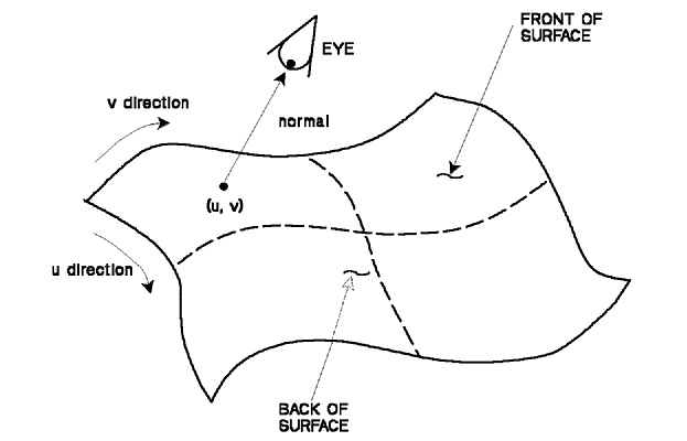
Surface primitives such as polygons and NURBS surfaces have a front side and a back side defined by the geometric normal of the surface. The normal is used when processing the surface for such operations as shading and culling.
Given a surface normal, the API uses the following rule to determine which side of the surface is the front:
If the tail of the geometric normal is placed on the surface, the front side is the one which is seen when sitting on the head of the normal looking toward the tail.
The figure, "Determining the front and back faces of a surface," illustrates the above rule.
The geometric normal may be specified by your application for some primitives or will be calculated by the graPHIGS API The geometric normal is usually the normal to the surface but your application can specify it otherwise. For planar primitives, the geometric normal is used in place of vertex normals when the vertex normals are not specified by your application. The method used by the graPHIGS API to calculate the normal will be described for each surface primitive, so that you will be able to predict which side of a primitive will be the front.
When you need or want to store, as one element, many related but unconnected line segments, use the Disjoint Polyline (GPDPL2 and GPDPL3) subroutines to create disjoint polyline structure elements. Disjoint polylines are similar to polylines in all respects except that they let your application store unconnected lines within a single primitive structure element.
Both GPDPL2 and GPDPL3 enable your application to draw a line segment, move to the next point without drawing, then draw a line segment within the same primitive. To accomplish this, the graPHIGS API accepts as input a move and draw array that specifies whether to draw a line segment from the current point to the next point or to move to the next point without drawing.
The figure, "Disjoint Polyline Data and Cube," shows the arrays used to draw the pictured cube with a single disjoint polyline outputprimitive.
Like the Disjoint Polyline Primitive, Polyline Set 3 with Data (GPPLD3) allows you to store as one element, many related but unconnected line segments. During traversal, these elements generate a sequence of polylines from the specified list of points. Polyline Set 3 with Data also allows you to specify color per vertex.
You can control the color of a line segment three ways: 1) through use of the current polyline color, 2) through the color of the associated vertex, and 3) by interpolating between the colors of the vertices at the endpoints of the line.
The first method requires no color definition beyond that which you specify for the polylines. For the second and third methods, you must specify vertex colors with the primitive. The third method also requires you to insert a Set Polyline Shading Method attribute. See "Set Polyline Shading Method"
Use Set Polyline Shading Method (GPPLSM) when you want a gradual change in color (interpolation) across polyline segments spanning vertices of different colors. If you are specifying that polyline shading color be used with GPPLSM, you must be sure to define vertex colors in the Polyline Set 3 with Data primitive.
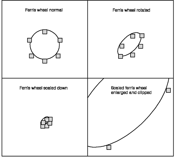
With the graPHIGS API, your application can control the color of individual pixels on a workstation display through the Pixel (GPPXL2 and GPPXL3) subroutines. Your application defines the color of each pixel as in index into the workstation's default color table. The default color table for most workstations is the display color table which implies that the content of this primitive is copied directly to the frame buffer. For more information on color tables, see Chapter 17. "Manipulating Color and Frame Buffers"
In addition to the array of pixel values, your application specifies a point in Modeling Coordinates (MC) at which to position the array of colors. That specified point corresponds to the top left corner of the pixel rectangle.
The figure, "The Pixel Output Primitive," shows how transformations affect only the location of the pixel data. Note that not all devices support clipping of the pixel primitive.
When a pixel primitive is encountered during structure traversal, each pixel index is written to the frame buffer in a workstation-dependent way depending upon the size of the workstation's frame buffer. For example, for an 8-bit frame buffer, the lower order 8-bits of each pixel index are written to the frame buffer. For a 24-bit frame buffer, the lower order 8-bits of each pixel value are duplicated in each component of the frame buffer. For more information on colors, frame buffers, and the color pipeline, see Chapter 17. "Manipulating Color and Frame Buffers"
The Circle 2 (GPCR2) subroutine lets your application create structure elements which define circles by specifying a circle's center point and a radius. The center point is specified in X and Y Modeling Coordinates and the Z coordinate is assumed to be zero. Your application can create a 3D circle using the ellipse subroutine. Circle primitives are drawn as polylines and are not filled.
The Circular Arc 2 (GPCRA2) subroutine lets your application creates a structure element which defines a circular arc (that is, a portion of a circle's perimeter). In addition to the arc's center point and radius, two angles are specified that define the portion of the circle's perimeter to be displayed. The arc is drawn in the counter-clockwise direction from the starting angle position to the ending angle position in the Z=0 plane.
The ellipse structure element defines an ellipses in either 2D or 3D Modeling Coordinates (MC) and can be created using the Ellipse 2 (GPEL2) or Ellipse 3 (GPEL3) subroutines. Ellipses are drawn as polylines and are not filled.
An ellipse is defined by a center point and two vectors originating from the center point. The magnitude and direction of the first vector define the major axis of the ellipse. The second vector defines a point on the perimeter of the ellipse. For GPEL2, the ellipse is drawn through the two points in the Z=0 plane. For GPEL3, the ellipse is drawn through the two points in the plane specified by the two vectors.
The elliptical arc GDPs (GPELA2 and GPELA3) let your application display a portion of the perimeter of an ellipse. The arc is defined by two parameter values that define the start and the end of the arc. The arc is drawn in the direction of increasing parameter values.
The following is the basic form of the parametric ellipse:
P(t) = A ū cos (t) + B ū sin (t) + C
where:
A is the vector defining a point on the ellipse relative to the center
B is the vector defining another point on the ellipse relative to the center
C is the vector defining the center of the ellipse
t is the parametric variable.
Note that A and B are not required to be orthogonal.
The drawing direction of an ellipse can be changed using one of the following methods:
The following table summarizes the parameters of this
equation for each of the graPHIGS API primitives:
| Full (closed) | Arc | |
|---|---|---|
| Ellipse | C = (Cx, Cy, Cz) A = (Ax, Ay, Az) B = (Bx, By, Bz) t1 = 0 t2 = 2 pi |
C = (Cx, Cy, Cz) A = (Ax, Ay, Az) B = (Bx, By, Bz) t1 = specified t2 = specified |
| Ellipse 2 | C = (Cx, Cy, 0) A = (Ax, Ay, 0) B = (Bx, By, 0) t1 = 0 t2 = 2 pi |
C = (Cx, Cy, 0) A = (Ax, Ay, 0) B = (Bx, By, 0) t1 = specified t2 = specified |
| Circle 2 | C = (Cx, Cy, 0) A = (r, 0, 0) B = (0, r, 0) t1 = 0 t2 = 2 pi |
C = (Cx, Cy, 0) A = (r, 0, 0) B = (0, r, 0) t1 = specified t2 = specified |
A polygon with data primitive is an extension of the polygon primitive that defines a polygon from a set of contours which can be rendered with one of several interior styles. In addition to the vertex coordinates and sub-area definitions, this primitive definition can include additional information to control the rendering process. For the two- and three-dimensional forms of this primitive, vertex colors, convexity flags, and boundary flags may be specified. The geometric normal of the polygon and/or a normal for each vertex may be specified for the three-dimensional form only. The specified colors and normals are used in rendering the primitive. For example, the normals may be used in the lighting calculations to produce more realistic effects.
The convexity flag indicates that the application has determined the convexity of the polygon to be either CONCAVE or CONVEX. As a result, the graPHIGS API does not have to determine the convexity of each polygon every time the primitive is rendered, and rendering performance is improved. Sample C subroutines for determining the convexity of a set of polygons is provided in The graPHIGS Programming Interface; under the following AIX directory:
/usr/lpp/graPHIGS/samples/convexcheck
Provided with the sample subroutines is a README file which explains their use.
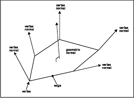
A polygon with data primitive is created by calling the Polygon with Data (GPPGD2 and GPPGD3) subroutines. The figure, "Five-sided polygon showing vertex normals and geometric normal," shows a polygon with vertex normals and a geometric normal.
Note that the normals do not have to actually be orthogonal (normal) to the polygon.
The edges of this primitive are the same as for polygon except when the boundary flags are specified. In this case, only a subset of the polygon's perimeter will comprise the edge. The Edge Flag attribute still has the same meaning for this primitive as for polygon, which is to control whether the defined edges are rendered or not. Notice that when the Edge Flag attribute is set to 1=OFF , the boundary flags have no effect. When it is set to 2=ON , only those parts of the polygon's perimeter defined by the boundary flags will be rendered as part of the edge.
As for polygon 3, it is the responsibility of your application to ensure that all vertices of the three-dimensional form of this primitive are co-planar. The effect produced by non-planar polygons is undefined.
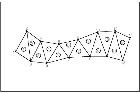
To create a triangle strip such as the one shown in the figure, "Triangle strip primitive," your application can call the Triangle Strip(GPTS3) subroutine. The triangle strip primitive generates a sequence of n-2 triangles from n vertices. The kth triangle is defined by vertices k, k+1 and k+2
As with polygon with data primitive, additional information may be specified to control the rendering of the primitive more precisely. Colors and normals may be specified for each triangle vertex as well as a geometric normal for each triangle.
The edges of this primitive are the line segments forming the boundaries of all triangles in the strip.
Note: Unexpected results may be produced on some workstations when a line type other than solid is selected.
To create a quadrilateral mesh primitive such as the one shown in the figure, "Quadrilateral Mesh Primitive," use the Quadrilateral Mesh 3(GPQM3) subroutine.
Note: This figure shows numbering of vertices for a 4 by 3 primitive.
The quadrilateral mesh primitive generates a sequence of m-1 by n-1 quadrilateral facets from m by n vertices. Each set of four neighboring vertices defines a quadrilateral. Thus, each vertex you specify, except those at the ends, is used by four different facets. In this way, the application makes more efficient use of your vertices than it does when generating triangle strips.
You are not required to specify that the vertices of each quadrilateral lie in the same plane, however, the method of rendering such a quadrilateral depends on the workstation used.
If you specify fewer than two vertices in either direction, then the primitive is not visible.
You may specify additional data to control such aspects of rendering as color and edges.
A character line primitive is created using the Character Line 2 (GPCHL2) subroutine. An integral number of a specific character is generated along a line between two end points by this primitive. It is classified as a text primitive and therefore uses most of the text attributes. The specification of this primitive includes the two end points, a nominal height in Modeling Coordinates and a single byte character code of the character to be used. Note that double byte characters cannot be used.
The current character set is bound to this primitive at definition time. The combination of text font, character set and character code at traversal time determine the actual set of strokes that are generated at each character position along the line. The actual height of the characters for a specific character line primitive will be the product of the nominal height from the primitive specification and a new attribute called character line scale factor. The character height attribute is ignored. As stated before, an integral number of characters is used to represent the line. As the character line primitive is scaled, the number of characters along the line will change but the height remains constant. The expansion factor is modified to ensure that an integral number of characters is produced and that there is no space at either end of the line segment. Text alignment and character spacing are not applied to this primitive. See the section "Character Line Attributes" for details.
A marker grid primitive defines a planar grid of markers. The two-dimensional form of this primitive creates the grid in the XY plane (Z=0.0) of Modeling Coordinate space. The three-dimensional form specifies an arbitrary plane in three space in which the markers will be positioned. To create a two-dimensional or three-dimensional marker grid, your application should call the Marker Grid 2 (GPMG2) or Marker Grid 3 (GPMG3) subroutines respectively.
Each position on the grid is defined by the following parametric vector equation:
Pi, j = P0 + iV1 + jV2
imin <= i <= imax
jmin <= j <= jmax
where:
+-Pi, j is the position of the marker at grid location i, j
P0 is a 2D or 3D modeling coordinate which defines the origin of the grid
V1 is a 2D or 3D vector that defines the location of grid location i+1, j relative to grid location i, j
V2 is a 2D or 3D vector that defines the location of grid location i, j+1 relative to grid location i, j
imin , imax are the limits for parameter i. Can be any integer (positive, negative or zero).
jmin , jmax are the limits for parameter j. Can be any integer (positive, negative or zero).
The parameters required to define a grid are then P0 , V1 , V2 and the limits on i and j (imin , imax , jmin , jmax ).
Be aware that marker grid primitives are subject to all transformations and can result in a large number of markers generated for a grid that is defined or transformed in three dimensions so it becomes parallel or near parallel to the direction of projection.
A line grid primitive is created using either the Line Grid 2 (GPLG2) or Line Grid 3 (GPLG3) subroutines and defines a planer grid of 2 groups of crossing line segments. The two-dimensional form of this primitive creates the grid in the XY plane (Z=0.0) of modeling coordinate space. The three-dimensional form specifies an arbitrary plane in three space in which the lines will be positioned.
A line segment is generated for each pair of endpoints (P1 , P2 ) for each value of i and j as shown in the following equations:
Line segments parallel to V1 :
P1 (j) = P0 + imin V1 + jV2
P2 (j) = P0 + imax V1 + jV2
Line segments parallel to V2 :
P1 (i) = P0 + iV1 + jmin V2
P2 (i) = P0 + iV1 + jmax V2
where:
jmin <= j <= jmax
imin <= i <= imax
P1 , P2 = Endpoints of lines inthe grid.
P0 = a 2D or 3D modelling coordinate which defines the origin of the grid.
V1 = a 2D or 3D vector that defines the direction of the i grid lines and the relative spacing of the j grid lines.
V2 = a 2D or 3D vector that defines the direction of the j grid lines and the relative spacing of the i grid lines.
imin , imax = limits forparameter i. They can be any integer, positive, negative or zero.
jmin , jmax = limits forparameter j. They can be any integer, positive, negative or zero.
The parameters required to define a grid are then P0 , V1 , V2 and the limits on iand j (i(sub min), i(sub max), j(sub min), j(sub max)). This primitive is subject to all transformation and clipping and all polyline attributes are used in rendering it.
Be aware that a large number of lines may be generated for a grid that is defined or transformed in three space so that it becomes parallel or near parallel to the direction of projection.
The Annotation Text Relative primitive (GPANR2 and GPANR3) define annotation text associated with a specified reference point. Using this primitive with the Set Annotation Style (GPAS) attribute, a line can be drawn from the reference point to the annotation text origin.
The transformation pipeline transforms the specified reference point to NPC coordinates. If the resulting point is clipped, then no annotation text is displayed. If the reference point is not clipped, then the annotation text is positioned relative to the reference point, as specified by the text vector. The rendering consists of the specified annotation text and an annotation style. Text is drawn using the offset specified by the text vector as the origin of the text coordinate system, and is drawn as normal annotation text using the current annotation traversal attribute values. Annotation style is controlled by the Set Annotation Style attribute. If the attribute is set to LEAD_LINE , a line is drawn from the reference point to the text origin, using the current polyline traversal attribute values. When drawn, the text string and the annotation style rendering are subject to the normal clipping rules (as long as the reference point is not clipped.)
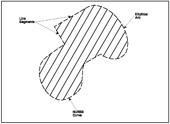
A composite fill area primitive is created by calling the Composite Fill Area 2 (GPCFA2) subroutine and is defined by the following line geometry forms:
Note: Circular Arcs are a subset of these.
The specified geometry segments define the contours of the fill area as shown in the figure, "Composite fill area definition." The curves of each contour must be explicitly connected and each contour must be explicitly closed by connecting the last curve to the first. However, any gaps due to floating point inaccuracies will be closed implicitly.
The polygon attributes including lighting and shading are used to render this primitive.
The composite fill area primitive may contain multiple loops in its boundary definition, similar to a polygon primitive.
The parameters your application must supply to the GPCFA2 routine are:
The drawing direction of each segment of the primitive is important in order for the geometry segments to meet properly. For example, a NURBS curve is drawn from the minimum parameter value to the maximum parameter value. The geometry segments drawn before and after a NURBS curve must meet the curve at its start and end points respectively. In order to reverse the drawing direction of a NURBS curve your application must reverse the order of the control points and adjust the knot vector accordingly. To reverse the direction of an elliptical arc, see the definition of the elliptical arc primitive presented earlier in this chapter.
A polyhedron edge primitive is created by calling the Polyhedron Edge (GPPHE) subroutine and is used to represent the intersection of two planes or faces of a polyhedron type object. Multiple intersections may be specified within the same structure element. The definition of each edge segment requires the two end points of the edge and the two normals of the faces or planes whose intersection has created the edge.
The normals are used to control whether or not the line segment is actually rendered. When it is rendered, the polyline attributes are used.
A polyhedron primitive is used to model polyhedron objects in which some of the edges are considered sharp and others are only construction lines. This primitive can be used to produce various effects when modeling polyhedron objects as discussed in the Chapter 16. "Rendering Pipeline"
A polysphere structure element is created using the Polysphere (GPSPH) subroutine. When drawn, a polysphere structure element will generate a set of spheres each defined by a center point and a radius. The polysphere primitive is an area defining primitive, therefore, polygon attributes and surface attributes apply to the interior of the polysphere. In addition, polyline attributes and surface attributes apply to the tesselation curves of the polysphere.
Because a sphere has no edges, polygon edge attributes do not apply to this primitive, and boundaries are not drawn. A sphere with Interior Style of HOLLOW does not have a direct effect on the display, except when HLHSR processing is active. During HLHSR processing, such a sphere is rendered into the Z-buffer, so a hollow sphere hides parts of other primitives that are farther away in their Z extent. Workstation-dependent techniques are used to perform highlighting color and pick echo for hollow and empty interior styles.
The polysphere primitive is ideal for such applications as molecular modeling and provide better performance than a NURBS surface shaped as a sphere.
The PHIGS PLUS standard and the associated graPHIGS API extensions allow curves and surfaces to be defined in terms of Non-Uniform Rational B-Splines (NURBS). With the appropriate choice of hardware architecture and software algorithms, rendering curved surfaces defined as NURBS is faster and more accurate than rendering the same surfaces defined by polygons.
There are a number of characteristics which must be understood in order to use NURBS curves and surfaces effectively. These include specification of the data representing curves and surfaces, as well as transformation, tessellation, and evaluation of NURBS curves and surfaces.
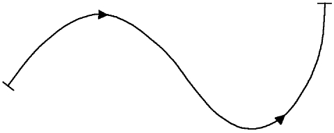
This section focuses on the characteristics and generation of NURBS entities from the graPHIGS API point of view. These entities consist of 2D parametric curves, 3D parametric curves, simple (untrimmed) parametric surfaces, and trimmed parametric surfaces. The figure, "A 2D NURBS curve," provides a simple example of a 2D NURBS curve.
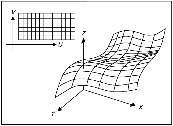
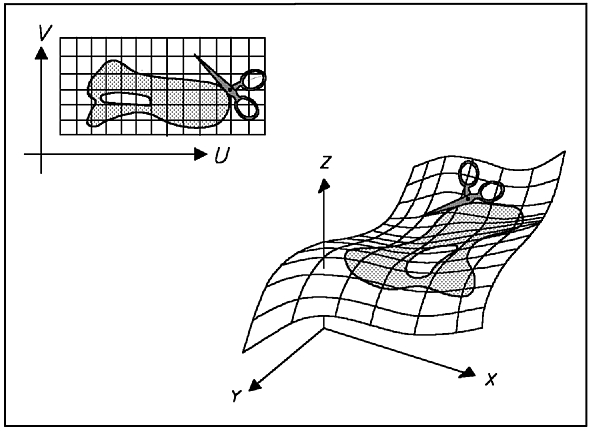
A NURBS surface consists of a 2D rectangle which may be bent, stretched, and twisted to form a 3-D shape. A simple or untrimmed NURBS surface, as shown in the figure, "A NURBS Surface," consists of the entire rectangular surface which has been formed into a 3D shape. A trimmed NURBS surface, as shown in the figure, "A Trimmed NURBS Surface," is similar to a dress pattern where the trimming curves define the pattern to be cut out of the surface. One or more NURBS curves may be specified within the rectangular area which defines the surface. Any portions of this surface outside these curves are discarded. Anything bounded by an even number of curves, such as the interior of the hole shown in the figure, "A NURBS Surface," is also discarded. The resulting 3D surface includes everything bounded by an odd number of curves.
Note: In the figure, "A Trimmed NURBS Surface," the upper diagram represents trimming curves defined in the surface coordinates. The lower diagram represents the resulting 3D trimmed surface.
The following section reviews the essential characteristics of NURBS curves and surfaces. This will be followed by a discussion of tessellation, the process which controls the accuracy with which a curve or surface is rendered. Finally, we will examine how NURBS have been implemented as graPHIGS API primitives.
In addition to the geometric coordinates (x,y,z), NURBS depend on one or two parametric coordinates (t, or u and v) which increase monotonically from the start of a curve to the end, or from one edge of a surface to the opposite edge. Thus, for 3D curves, we have:
x = X(t)
y = Y(t) for tmin <= t <= tmax .
z = Z(t)
where: X(t), Y(t), and Z(t) are functions of the parametric coordinate t. Likewise for surfaces, we have:
x = X(u,v)
y = Y(u,v) for umin <= u <= umax ,
z = Z(u,v) and vmin <= v <= vmax .
In addition, for trimmed surfaces, the boundary curves are defined as:
u = U(t)
v = V(t) for tmin <= t <= tmax .
NURBS are closely related to other types of parametric functions, such as Bezier functions, which are actually a special case of NURBS. Parametric curves and surfaces may also be defined in terms of simple polynomials, and any such parametric polynomial function may be represented exactly by a corresponding NURBS function.
NURBS curves and NURBS surfaces may be defined in either rational (hence the R in NURBS) or non-rational forms. In the simpler non-rational form, each component (x, y, or z) of a NURBS curve, for example, may be determined by evaluating a polynomial function of the parametric coordinate:
| m | ||
| X(t) = | |
cxi ti |
| i=0 |
| m | ||
| Y(t) = | |
cyi ti |
| i=0 |
| m | ||
| Z(t) = | |
czi ti |
| i=0 |
The rational case is similar, except that there is an additional function called the weight, which is defined as follows:
| m | ||
| W(t) = | |
cwi ti . |
| i=0 |
In this case, the geometric coordinates are determined by ratios of polynomials:
X(t) = WX(t) / W(t),where: WX(t) , WY(t) , and WZ(t) are polynomials similar those which specify X(t) , Y(t) , and Z(t) for the non-rational case.
Each NURBS function, like any polynomial, may be characterized by the degree (m) corresponding to the highest power of the parametric coordinate. Equivalently, a NURBS function may be characterized by the order (k=m+1) corresponding to the number of linearly independent terms in a polynomial of degree m Thus a linear function has degree 1 and order 2, a quadratic function has degree 2 and order 3, and so forth.
Unlike a simple polynomial function, for which a single set of coefficients (ci , i = 0 to m) characterizes the entire function, a NURBS function may be represented by multiple sets of coefficients, each of which is valid only for a limited range of the parametric coordinate. Thus, a curve may be divided into a sequence of spans, each represented by different polynomials. This is illustrated by the curve in the figure, "The piecewise polynomial representation of a curve," which consists of three spans.
Note: This curve is determined by the six polynomials x1 , y1 , x2 , y2 , x3 , and y3 .
The first span is defined by parameter values t running from t0 to t1 . The coordinates of this portion of the curve are determined by the following polynomials:
| k | ||
| X1 (t) = | |
cx1i ti , and |
| i=0 |
| k | ||
| Y1 (t) = | |
cy1i ti . |
| i=0 |
The second span, defined by parameter values running from t1 to t2 , is determined by the following polynomials:
| k | ||
| X2 (t) = | |
cx2i ti , and |
| i=0 |
| k | ||
| Y2 (t) = | |
cy2i ti . |
| i=0 |
Likewise, the third span, with parameter values running from t2 to t3 , is determined by the following polynomials:
| k | ||
| X3 (t) = | |
cx3i ti , and |
| i=0 |
| k | ||
| Y3 (t) = | |
cy3i ti . |
| i=0 |
The parametric polynomials that describe adjacent spans of a NURBS curve are defined so as to provide a specific degree of continuity, where degree 0 means the values are continuous, degree 1 means the value and first derivative are continuous, and so forth. The maximum degree of continuity is k-2 where k is the order of the functions. For example, a cubic curve (with degree m=3 and order k=4) may have spans joining with continuity of degree 2 (continuous second derivatives). A lower degree of continuity may be obtained by constructing the knot vector as discussed in the next section.
NURBS are defined by control points, weights, and knot vectors. The control points provide the primary control over the geometry of a curve or surface. A curve may have n control points, where n must be greater than or equal to the order k of the curve. A surface has an nu by nv matrix of control points where nu >= ku and nv >= kv , and ku and kv are the orders of the u and v parameters.
A NURBS curve or surface does not pass through (interpolate) the control points, except in certain special cases. Instead, the curve or surface merely passes near these points, as shown in the figure, "A NURBS curve and its control points," in which the curve passes near the control points, but not through them. If needed, it is possible to construct a NURBS curve which interpolates a set of n points, and the resulting curve is determined by a set of n control points which is related to the n interpolated points by a simple nxn matrix.
The weight values are optional and are used to define the rational form of the NURBS curves and surfaces. In this form, there is a weight value (w) associated with each of the control points (x,y,z). The weights and coordinates are combined to form the homogeneous coordinates (WX , WY , WZ , W ), which form the control points for a set of four parametric polynomial functions WX(t), WY(t), WZ(t), and W(t). The resulting geometric coordinates are determined by the following ratios:
x(t) = WX(t) / W(t)Similar expressions can be defined for surfaces. Consequently, each point is determined by a ratio of polynomials. In order to maintain a well behaved set of operations, the weights are required to be positive definite (must be greater than zero). The values of the weights are usually close to unity, and the rational form reduces to the non-rational form if the weights are all equal.
The knot vectors define a partitioning of the parameter space for the parametric coordinates t (for a curve), or u and v (for a surface). The knot vector for a curve of order k with n control points will have (n+k) components, of which the first and last are never used. Each span in the curve depends on 2 * m successive knot values, where m=k-1 and k is the order of the curve.
For a surface, there is a knot vector and a sequence of spans for each of two parametric coordinates. The portion of a surface determined by one span for each parameter is called a patch
If the values of the knots are spaced uniformly (for example, 0, 1, 2, 3, ...), then the result is called a uniform B-spline. For a non-uniform B-spline, the knot values may be separated by irregular intervals, and knot values may be repeated, as in the knot vector (0.0, 1.2, 1.5, 1.5, 2.7, 9.0).
As indicated previously, a curve of order k may be continuous up to degree k-2. A lower degree of continuity may be obtained by using repeated knot values in the knot vector. For example, a NURBS curve of order 4 (cubic) with no repeated knot values will be continuous first and second derivatives (degree 2 continuity). If a knot value is repeated so that the same value appears twice in a row in the knot vector, then the second derivatives will be discontinuous at the point where the parametric coordinate has the repeated value.
In this case, the function and first derivative would still be continuous. If a knot value is repeated twice (same knot value three times), then the first derivatives may be discontinuous, and the curve could have a sharp corner at this point. If a knot value occurs four times (or more), then the curve itself may be discontinuous.
The ability to match successive spans with a specified degree of continuity makes it possible to construct a complex curve passing through many points using low order NURBS. This property is extremely valuable because it makes it possible to avoid high order functions. High order functions, whether NURBS, simple polynomials, or any other type tend to be costly to evaluate and prone to numerical instabilities. High order polynomials often require double precision (64-bit) floating point operations for reliable evaluation, whereas low order NURBS may be evaluated with single precision (32-bit) arithmetic without loss of accuracy.
NURBS curves and NURBS surfaces all share certain fundamental features. These features are responsible for the selection of NURBS as the means of representing curved lines and curved surfaces in the graPHIGS API As a tool for geometric modeling, NURBS provide the following:
The following paragraphs provide a closer look at each of these characteristics. These paragraphs will use 2D curves to provide simple examples of each property. In most cases, the generalization to 3D curves and surfaces is very simple.
The local shape control means that each control point and each knot value influences or controls the shape of only a limited portion of a curve or surface. Each control point of a curve affects up to k spans, and each knot value affects up to 2 * m spans, where k is the order of the curve and m = k - 1 is the degree of the curve. Each control point for a surface with orders ku and kv affects a set of up to ku ū kv patches.
For example, if the first control point for the curves is moved, then the first span (t2 < t < t3) will change, but the second span (t3 < t < t4) and the third span (t4 < t < t5) will not change.
The local shape control property may be compared to the global control found when fitting a single high order polynomial to a number of points. For example, consider a polynomial of order 12 that passes through a a set of 12 data points. If any point is altered, the entire curve changes. Changing the starting point will change the way the curve approaches the ending point. If a cubic NURBS curve is determined by a set of 12 control points, then the first control point will influence only a short section of the curve near the first point. The remainder of the curve does not depend on the location of the first point.
NURBS can provide exact representations of the conic sections and quadric surfaces. The conic sections include circles and ellipses, as well as parabolas and hyperbolas. The quadric surfaces include the cylinder, cone, sphere, ellipsoids, hyperbolic paraboloid, and so forth. This class of curves and surfaces, especially the circle, cylinder, cone, and sphere, are essential for geometric modelling, especially in CAD/CAM applications. The exact representations of these shapes require the rational form of the NURBS with the associated weight values. This is the principal reason for generalizing parametric curves and surfaces to the rational form, and the principal reason for the support of these rational forms as part of the graPHIGS API
The tables on Supported Primitives indicate how to specify the control points and weights for a circle. The geometry of these points is shown in the figure, "The control points for a circle." This is only one of an infinite number of ways to define a circle with NURBS. Similar sets of points and weights may be used to construct spheres, cylinders, and so forth.
Note: In the figure, "The control points for a circle," nine control points, along with the weight values specified in Table 1, are used to define a circle with radius R centered at (Xc, Yc). The knot vector for this curve is (0,0,0,1,1,2,2,3,3,4,4,4).
Table 5. The 2D circle as a NURBS curve. The
following nine sets of control points and weights may be used to generate a
circle with radius R centered at (Xc,Yc).
| point | X-ctrl | Y-ctrl | weight |
|---|---|---|---|
| 1 | Xc + R | Yc | 1 |
| 2 | Xc + R | Yc + R | 1/sqrt(2) |
| 3 | Xc | Yc + R | 1 |
| 4 | Xc - R | Yc + R | 1/sqrt(2) |
| 5 | Xc - R | Yc | 1 |
| 6 | Xc - R | Yc - R | 1/sqrt(2) |
| 7 | Xc | Yc - R | 1 |
| 8 | Xc + R | Yc - R | 1/sqrt(2) |
| 9 | Xc + R | Yc | 1 |
NURBS curves and NURBS surfaces are contained within the convex hull of their control points. The convex hull is the smallest convex polygon (2D case) or smallest convex polyhedron (3D case) which contains a given set of points.
This property applies to each span of a curve and each patch of a surface, as well as to a complete curve or surface. That is, each span of a curve must lie within the convex hull of the k control points which define that span, where k is the order of the curve. Likewise, each patch of a surface is contained within the convex hull of a set of ku by kv points, where ku is the order of the u parameter and kv is the order of the v parameter.
This property makes it possible to make estimates of and place bounds on the size and location of a NURBS curve or surface without evaluating a single point. An important application of this property is found in trivial rejection testing. If the convex hull does not overlap with the current screen or window, then the surface is not evaluated. This has a large effect on the performance of a system when a user zooms in for a detailed view of a small portion of a complex scene or object. In this case, most of the surfaces can be rejected, allowing the display to be updated rapidly. Similar advantages are obtained when processing a NURBS curve or surface for pick input.
There are several efficient algorithms for evaluating NURBS functions. In principle, the control points and knot values for a NURBS function may be used to determine the coefficients of the corresponding polynomials for each span. These may then be evaluated using Horner's Rule:
| m | ||
| f(t) = | |
ci ti |
| i=0 |
| = C0 + t(C1 + t(C2 + ...)) |
This requires only m multiplications and m additions per point. Calculation of the coefficients, however, may cost more than evaluating a number of points. In addition, the coefficients in this sum frequently have large magnitudes with opposing signs. Consequently, the result may be very sensitive to round-off and truncation errors in the floating-point operations. In this case, the intrinsic numerical stability characteristic of NURBS has been destroyed by converting to the polynomial representation. Thus, even though NURBS may be formally equivalent to certain polynomials, it is usually best to avoid any explicit reference to these polynomials when processing a NURBS function.
An alternative to Horner's Rule is provided by the forward difference method. This is frequently used for Bezier curves which are a special case of NURBS. In this case, the control points are used to determine a set of forward difference components, di, which are related to successive derivatives of the curve. Each point is evaluated by adding each component to its lower order neighbor:
di = di + di+1 , for i = m-1, m-2, ..., 0.
The resulting values of d0 form successive values of the function. This requires only m additions, and no multiplications, making this a very efficient algorithm on a point-by-point basis. This efficiency is partly offset by the cost of computing the first set of forward difference components, di. In addition, each point is based on the value of the previous point, and is subject to the cumulative effects of the limited precision of the floating-point operations in all preceding points within a span. Although these errors will usually be small, they may lead to gaps between successive spans of a curve, or rips between patches of a surface.
A third algorithm, called the DeCasteljau or Cox-DeBoor algorithm, is based on recursively interpolating the control points, as shown in the figure, "The Cox-DeBoor (DeCasteljau) algorithm for a cubic curve (order=4)." Intermediate points A, B, and C are interpolated between control points 1, 2, 3, and 4 based on the parameter value and the knot vector. Intermediate points D and E are interpolated between points A, B, and C in a similar manner. Point F on the curve is interpolated between points D and E. Segment DE is tangent to the curve.
One point on a cubic curve (order 4) would be given by the following operations:
f1
= ((a1
- t) Q1
+ (t - b3
) Q2
) / (a1
- b3
)
f2
= ((a2
- t) Q2
+ (t - b2
) Q3
) / (a2
- b2
)
f3
= ((a3
- t) Q3
+ (t - b1
) Q4
) / (a3
- b1
)
f1
= ((a1
- t) f1
+ (t - b2
) f2
) / (a1
- b2
)
f2
= ((a2
- t) f2
+ (t - b1
) f3
) / (a2
- b1
)
f(t) = ((a1 - t) f1 + (t - b1 ) f2 ) / (a1 - b1 )
where Q1 ... Q4 are four control point values, a1 , a2 , and a3 are the three knots following the parameter t, b1 , b 2 , and b3 , are the three knots preceding the parameter t, and f(t) is the result. The denominators are independent of t and the value of 1/(a1 - b1 ), for example, needs to be computed only once for each span.
This method requires on the order of m2 floating-point operations, compared to order m operations for Horner's Rule and forward differences. This penalty is not severe for small m (e.g. m = 3 or cubic functions), and is largely offset by reduced set-up cost (the control points are used directly). The interpolation formulas preserve the numerical stability of the NURBS functions, and each point is computed independently, so there are no cumulative errors as the calculations progress across a span. Consequently the last point on a curve will be just as accurate as the first, and each span will match the next with maximum accuracy.
A critical step in the processing of ordinary vectors and polygons is the transformation (rotation, translation, scaling, etc.) from Modelling Coordinates (MC) to screen coordinates or Device Coordinates (DC). Much attention has been devoted to developing specialized hardware for performing this process as efficiently as possible. With NURBS, such transformations may be applied to either the points (vertices) generated by evaluation of the NURBS functions, or to the control points which define a NURBS curve or surface. In both cases the results are exactly the same. The number of control points, however, is usually much less than the number of vertices generated by the evaluation of the NURBS. Consequently, it is much more economical to transform the control points than to transform the resulting vertices.
Transforming the control points instead of the vertices has two additional advantages. First, the transformed control points may be used for trivial rejection based on the convex hull property. In addition, if the curve or surface is not rejected, then the number of vertices generated to represent a curve or surface will usually be much greater than the number of control points. Consequently, the processing of vertices, including evaluation of the NURBS, is more critical for performance than the transformation of the control points. In this case, the transformation of the control points may be pulled away from specialized transformation hardware and performed on a slower general purpose processor. The specialized processors normally used for transformations of vertices may then be used to accelerate the evaluation of the NURBS. This assumes that the specialized transformation hardware is not so highly specialized that it cannot be used for anything else.
NURBS curves and NURBS surfaces form very compact data structures for representing complex shapes. A typical NURBS surface may be determined by roughly 10 to 100 control points with 12 to 16 bytes of data for each control point depending on whether or not the rational form is being used. Thus, the total amount of data needed to define a NURBS surface may be in the range of 1k to 2k bytes.
If a graphics workstation (or display station) does not support NURBS, then the same surface may be approximated with a grid of polygons. The number of polygons required to represent a given surface depends on the accuracy or quality expected for the resulting images. This number must be sufficiently large to produce a satisfactory image at the largest scale at which the surface is to be displayed. These conditions may usually be satisfied with 100 to 1000 four-sided polygons. To support smooth shading, the coordinates (x, y, z) for each vertex must be accompanied by the corresponding surface normal (Nx, Ny, Nz), yielding a total of 24 bytes per vertex or roughly 100 bytes per polygon. As a result, it may require 10k to 100k bytes to approximate the same surface defined exactly by only 1k to 2k bytes of NURBS data.
As an example, a set of 17 NURBS surfaces can be used to closely approximate a jet aircraft. All together, these 17 surfaces require less than 18k bytes of data. When represented with polygons at a medium level of quality, the same surfaces require roughly 5000 4-sided polygons occupying over 500k bytes, or more than 25 times as much data as required by the NURBS surfaces.
The amount of data required to represent a surface as polygons may be reduced by a factor of from 2 to 4 by combining the polygons into more efficient data structures such as triangle strips or a quadrilateral mesh. On the other hand, the amount of data required for the polygons may also be increased by similar or larger factors by tightening the requirements for how well the polygons must approximate the true curved surfaces. Consequently, we see that the amount of data required to represent a object with NURBS is 10 to 100 times smaller than that required to represent the same object with polygons.
Because of the data compression inherent in NURBS, it is clear that NURBS are of great value as a data communications tool, as well as a graphics tool. Using NURBS instead of polygons is equivalent to increasing the host to workstation data transfer rate by a factor of 10 to 100. In addition, this same data compression factor means NURBS make much better use of system resources such as real memory and mass storage than the corresponding polygon data. This can translate into the ability to support more complex graphics, such as a comparison of ten different airplanes. In addition, this can influence performance by controlling whether a complex model resides mainly in cache, real memory, local mass storage, or even on a remote host.
Tessellation is the process by which a curved line is divided into segments that may be approximated with straight lines, or a curved surface is divided into areas that may be approximated with flat polygons. Ideally, tessellation would not be needed. A curved line, for example, would be drawn as a sequence of points or pixels determined directly by the control points and/or other data defining the curved line. Lacking this capability, the workstation may divide a curved line into straight vectors (or anything else it can draw) in any manner as long as any resulting errors are negligible, such as less than one pixel.
Currently, however, there are several obstacles to this ideal. First, the judgement of what constitutes a negligible error is not uniquely defined. Secondly, even when a measure of error has been selected, as well as the size of this error which is considered to be negligible, the problem of determining how to satisfy these conditions can be more complex than the problem of evaluating the curve (or surface) at the selected points. Finally, the performance of current workstations tends to be strongly influenced by the size of the acceptable errors and the resulting number of points at which a curve or surface is evaluated.
The graPHIGS API permits the quality/performance trade-off to be controlled by allowing your application program to select how the error will be measured and the size of the acceptable error. In the case of NURBS curves, the measure of error is determined by the "curve approximation criterion", and the error tolerance is determined by a curve approximation control value. The recognized approximation criteria include:
In the first case, the control value specifies the number of steps into which each span is to be divided. In the case of the metric criterion, the control value may indicate the maximum length of any segment in pixels. The chordal deviation is based on the distance between the true curve and the straight segments used to approximate the curve.
A similar set of criteria are defined for curved surfaces, except that there are two control values, one for each parametric coordinate. In addition, there is a set of corresponding criteria for the trimming curves for trimmed surfaces. These criteria are all defined as attributes, analogous to colors, line styles, polygon interior styles, and so forth.
The graPHIGS API supports the following three criteria for tessellation of curves and surfaces:
Criterion 1 is based on the chordal deviation in Device Coordinates (DC). This method automatically adjusts the number of intervals in each span based on the curvature of the span and the scale of the figure. Criterion 1 is the criterion to use for all but a few unusual situations.
Criterion 3 specifies that each span (or each edge of each patch) is to be divided into a fixed number of intervals without regard to the curvature or scale of the figure. This criterion is provided for compatibility with PHIGS+.
Criterion 8 is an extension to the criteria defined in PHIGS+. This method permits an application to supply a tessellation vector which may represent any criterion an application may choose to define. Each component of the tessellation vector (specified as part of the data for a curve or surface) is proportional to the number of intervals for one span of a curve or one edge of a surface patch. This permits the tessellation to be custom-tailored by any application requiring exceptional treatment of curves or surfaces. This is the advanced option which would enable skilled programmers to substitute their own algorithm for the built-in algorithm used by the graPHIGS API for criterion 1.
In order to obtain the maximum performance, a tessellation algorithm will seek to evaluate a curve or surface at the minimum number of points required to satisfy the corresponding approximation criterion. In striving to meet this objective, however, a tessellation algorithm must also avoid the creation of "artifacts" such as pinholes (isolated missing pixels) or rips (sequences of missing pixels) in a surface. Such artifacts will occur, for example, if a surface is first divided into patches, and then each patch is tessellated independently. In this case, the vertices of the polygons which approximate the surface on one side of a patch boundary will not coincide with those on the other side. This creates small triangular holes along the boundaries between adjacent patches. The resulting artifacts can be very distracting when they permit a background of one color to show through holes in a surface of a sharply contrasting color. The API eliminates these artifacts by systematically tessellating each surface as a single entity.
The following paragraphs describe the support for NURBS curve and surface primitives within the graPHIGS API These structure elements are defined as Generalized Drawing Primitives (GDPs), and therefore may not be supported on all hardware platforms. To determine if the hardware your application is using supports NURBS curves and surfaces, use the Inquire List of Generalized Drawing Primitives (GPQGD) subroutine. The actual parameter limits of the subroutine calls discussed below should be inquired using the subroutines Inquire Curve Display Facilities (GPQCDF), Inquire Surface Display Facilities (GPQSDF), and Inquire Trimming Curve Display Facilities (GPQTDF)
Two-dimensional and three-dimensional NURBS curve structure elements can be generated with the Non-uniform B-spline Relational Curve 2 (GPNBC2) and Non-uniform B-spline Curve 3 (GPNBC3) subroutines respectively. The parameters for both subroutines are discussed below:
ti >=t(i - 1)
Note: If the curve approximation criteria is 1 and tessellation data is supplied, performance will be hindered due to the storage overhead of the tessellation data.
The parameters tmin and tmax are subject to the following restrictions:
To obtain a complete curve set tmin = tk and tmax = t(n + 1) .
The number of spans generated by GPNBC2 and GPNBC3 will be n - k. If fewer than k + 1 control points are specified, no curve will be generated.
A NURBS surface can be defined using the Non-Uniform B-Spline Surface (GPNBS) subroutine. The parameters for GPNBS are defined as follows:
The maximum surface order (max) supported can be inquired using the Inquire Surface Display Facilities (GPQSDF) subroutine.
A knot vector is subject to the following restrictions:
The knot vector has the following properties:
Typically, you should choose the following values for the first two and last two knots:
If the surface approximation criteria is 8 then the ith u span will be divided into Qu ū fui intervals and the v span will be divided into Qv ū fvi intervals where Qu and Qv are the control values supplied with the surface approximation criterion.
Note: If the surface approximation criteria is 1 and tessellation data is supplied, the performance will be hindered due to the storage overhead of the tessellation data.
The parameters umin, umax, vmin, and vmax are subject to the following restrictions:
To obtain the complete surface, set umin = uku, umax = u(nu + 1) , vmin = vkv, and vmax = v(nv + 1). . The number of surface patches generated by GPNBS will be unum - uorder by vnum - vorder. If unum or vnum is less than or equal to the order for the corresponding direction, no patches will be generated.
The edge for this primitive consists of the lines ofconstant parameter at the boundary of the surface.
Trimmed Non-Uniform Relational B-Spline surface primitives are generated using the Trimmed Non-Uniform Relational B-Spline Surface (GPTNBS) subroutine. The parameters for GPTNBS includes all the parameters of the Non-Uniform Relational B-Spline Surface primitive except the u and v parameter limits are specified as a set of curves comprising multiple contours called trimming curves The contours can be disjoint and can be contained inside one another to produce surfaces with holes. Trimming curves are similar to the edges of a polygon except that polygon edges are defined in three-dimensional modeling space while trimming curves are defined in the two-dimensional parameter space (u, v coordinates) of the surface.
Trimming curves may be any two dimensional non-uniform realational B-spline curve which adheres to the following guidelines:
If these guidelines are violated, the resulting display will be indeterminate.
The interior or "rendered" part of the surface is defined by the applying the odd winding rule within the its parameter space. This is the same rule used by the graPHIGS API to determine the interior of polygons.
In addition to the parameters specified for the GPNBS subroutine, the following information is required to specify trimming curves:
This section contains a discussion of the attributes applied to various primitives. The attributes are discussed according to the primitive group to which they apply. These groups are:
Each group is further divided into basic and advanced attributes. The basic attributes will only be described briefly as they are fully explained in Chapter 4. "Structure Elements"
Many of the attributes affect the color of primitives. There are two ways to define attribute colors; by an index into a color table or directly by specifying a color vector. A color vector consists of three color values that are interpreted based on the current direct color model. Your application can set the direct color model using the Set Direct Color Model (GPDCM) subroutine. For a complete discussion of the color pipeline, see Chapter 17. "Manipulating Color and Frame Buffers"
The following attributes are discussed in detail in Chapter 4. "Structure Elements"
The Set Highlighting Color Index (GPHCI) subroutine creates a structure element which sets the highlighting color for all subsequent primitives by specifying an index into the workstation's rendering color table.
The Add Class Name to Set (GPADCN) subroutine creates a structure element which adds the specified class names to the current class name set. All primitives in the structure created after a call to GPADCN will have the class name set as an attribute. Class names are integer identifiers used to make primitives invisible, highlighted, and pickable.
The Remove Class Name from Set (GPRCN) subroutine creates a structure element which removes the specified class names from the current class name set.
The Set Pick Identifier (GPPKID) subroutine creates a structure element which sets the current pick identifier for all subsequent primitives. Pick identifiers are part of the pick path information returned by a pick input device. For more information on pick devices and pick paths, see Chapter 7. "Input Devices" and Chapter 18. "Advanced Input and Event Handling"
The Set Highlighting Color Direct (GPHLCD) subroutine creates a structure element which sets the highlighting color for all primitives. (See "Frame Buffer Comparison Options" for a discussion of line-on-line highlighting used as a special rendering effect.) This attribute element is similar to the Highlighting Color Index element except that the color is specified with a color vector instead of an index into the rendering color table.
The Set Color Processing Index (GPCPI) subroutine creates a structure element which sets the current color processing method by specifying an index in the workstation's color processing table. (See "Frame Buffer Comparison Options" for a discussion of line-on-line highlighting used as a special rendering effect.) An application can use the Inquire Color Processing Facilities (GPQCPF) subroutine to determine the number of color processing method table entries available. For a complete description of color processing, refer to Chapter 17. "Manipulating Color and Frame Buffers" and Chapter 16. "Rendering Pipeline"
The Set Depth Cue Index (GPDCI) subroutine creates a structure element which sets the current depth cue information by specifying an index into the workstation's depth cue table. An application can use the Inquire Depth Cue Facilities (GPQDCF) subroutine to determine the number of entries in the depth cue table. For a complete description of depth cueing, refer to Chapter 16. "Rendering Pipeline"
The Set HLHSR Identifier (GPHID) subroutine creates a structure element which sets the current Hidden Line / Hidden Surface Removal (HLHSR) mode. The valid HLHSR identifiers are:
1=VISUALIZE_IF_NOT_HIDDENFor a complete description of Hidden Line/Hidden Surface Removal, refer to Chapter 16. "Rendering Pipeline"
The Set Antialiasing Identifier (GPAID) subroutine creates a structure element that indicates whether antialiasing is to be performed by the workstation. Antialiasing reduces the jagged appearance of objects drawn on raster displays by using techniques that "blur" the pixels to a more uniform appearance. Antialiasing techniques are workstation dependent, and not all workstations provide antialiasing capability. Refer to the workstation description information in The graPHIGS Programming Interface: Technical Reference for a description of available antialiasing methods and restrictions. Use the Inquire Available Antialiasing Mode (GPQAMO) to determine the antialiasing capabilities of your workstation. The application may control the antialiasing identifier attribute using the Set Extended View Representation (GPXVR) subroutine. This subroutine lets you specify that the antialiasing identifier be ignored (1=OFF ) or applied (2=SUBPIXEL_ON_THE_FLY ) or (3= NON_SUBPIXEL_ON_THE_FLY ) in the specified view.
The Set View Index (GPVWI) subroutine creates a structure element which changes certain current traversal values to those specified in the view table entry. This function provides compatibility with the ISO PHIGS standard. For best results, use this subroutine only if your application is already written to the ISO PHIGS standard, and avoid it if your application uses the graPHIGS subroutines for viewing (e.g. Associate Root To View (GPARV) and Set View Priority (GPVP)
The polyline attributes apply to the following primitives:
Polyline 2/3The basic polyline attributes, defined in detail in the first part of this guide, are reviewed in the following paragraphs.
The Polyline End Type (GPPLET) subroutine creates a structure element which sets the polyline end type to either flat, round, or square.
The Set Polyline Index (GPPLI) subroutine creates a structure element which is an index into a workstation polyline bundle table.
The Set Linetype (GPLT) subroutine creates a structure element which sets the polyline line type by specifying an index in the workstation's line type table.
The Set Linewidth Scale Factor (GPLWSC) subroutine creates a structure element which sets the polyline line width scale factor. The line width scale factor attribute is used to define the width of polyline primitives as a fraction of the workstation's nominal line width.
The Set Polyline Color Index (GPPLCI) subroutine creates a structure element which sets the polyline color by specifying an index in the workstation's rendering color table. For more information on the processing of colors, see Chapter 17. "Manipulating Color and Frame Buffers"
The Attribute Source Flag Setting (GPASF) subroutine creates a structure element which sets the attribute source flags for polyline line type, line width scale factor, and color attributes. Each attribute source flag controls whether a specified polyline attribute will be selected from individual attribute elements or through the workstation's polyline bundle table.
The advanced attributes applied to polyline primitives include the following:
Set Polyline Color Direct (GPPLCD) creates a structure element which sets the line color for all polyline primitives. This attribute element is similar to Set Polyline Color Index (GPPLCI) except that the color is specified with a color vector instead of an index into the rendering color table.
The Set Polyhedron Edge Culling Mode (GPPHEC) subroutine creates a structure element which controls the display of polyhedron edges. (This attribute applies only to the Polyhedron Edge (GPPHE) primitive.) Polyhedron edges are either front-facing or back-facing, depending on the transformed normals specified in the Polyhedron Edge primitive. You can control culled (not displayed) edges, using different settings of the culling mode attribute. You can specify culled edges if both normals are back-facing (2=BOTH_BACK ), front-facing (3=BOTH_FRONT ), facing the same direction (4=BOTH_BACK_OR_FRONT ), face different directions (5=BACK_AND_FRONT ), or if one normal is back-facing (6=LEAST_ONE_BACK ) or front-facing (7=LEAST_ONE_FRONT ). The Inquire Advanced Attributes Facilities (GPQAAF) subroutine returns which polyhedron edge culling modes are supported on a specified workstation.
Morphing modifies the geometry and/or data (texture) mapping data of a primitive. There are two types of morphing, one using vertex coordinates and the other using data mapping data values. These functions are called vertex morphing and data morphing, respectively. Because data morphing applies to area primitives only, data morphing cannot be used for polylines. Vertex morphing takes place in modeling coordinates. You define the changes using morphing values at each vertex of the affected primitives along with scale factors that define how the vertex morphing values affect the primitive. Use the Set Vertex Morphing Factors (GPVMF) subroutine to specify the scale factors. For more detailed information on vertex morphing, see "Morphing" Use the Inquire Workstation Description (GPQWDT) call to determine whether your workstation supports the graPHIGS API morphing facilities.
The modeling clipping function provides a way to clip geometric entities in world coordinates. The clipping volume in world coordinates is set by the Set Modeling Clipping Volume 2/3 (GPMCV2) and (GPMCV3) elements. Modeling clipping is activated or deactivated by the Set Modeling Clipping Indicator (GPMCI) element. Use the Inquire Workstation Description (GPQWDT) subroutine to determine whether modeling clipping is supported on your workstation. See "Modeling Clipping" for more information.
The Set Curve Approximation Criteria (GPCAC) subroutine creates a structure element which sets the curve approximation criteria for subsequent NURBS curves. GPCAC controls the tessellation of curves and applies only to the Non-Uniform B-Spline Curve 2/3 primitives. Tessellation is the division of each span into intervals which can be drawn as straight lines. The number of intervals used to represent each span is determined by the criterion and control value as summarized below:
(Criterion 1) WORKSTATION_DEPENDENT : The workstation-dependent curve approximation criterion relies on a control value Q which represents the quality of the curve approximation where 1.0 is nominal quality. A value of Q greater than or less than 1.0 produces a higher or lower quality curve respectively. Q is used to determine the number of tessellation intervals (n). The 6090 workstation uses a technique called chordal deviation to determine how close to approximate the curve. Chordal deviation is the perpendicular distance between the actual curve and the approximating line segment as shown in the figure, "Definition of chordal deviation." Chordal deviation is independent of modeling transformation.
(Criterion 3) CONSTANT_SUBDIVISION_BETWEEN_KNOTS : The simplest curve approximation criterion involves specifying a the number of subdivisions between knots as a constant N
(Criterion 8) VARIABLE_SUBDIVSION_BETWEEN_KNOTS : In the case of criterion 8, the number of tessellation intervals (n) is equal to the following: n = Q ū fi
where:
Q is the tessellation control value
fi is the ith tessellation data value supplied with the definition of the NURBS curve.
In addition to individual attributes structure elements, polyline attributes may also be controlled by bundle tables. The Set Extended Polyline Representation (GPXPLR) subroutine is an advanced version of the Set Polyline Representation (GPPLR) subroutine. Both subroutines allow your application to define bundle table entries for polyline attributes. Specifically, with GPXPLR your application can define polyline bundle table colors directly as color vectors as well as with a color index. To determine the number of entries in the bundle table, your application may use the Inquire Actual Length of Workstation State Tables (GPQALW) subroutine.
The Set Line Type Representation (GPLTR) subroutine allows your application to define line type entries in the workstation's line type table. To determine the number of entries in the line type table, your application can use the Inquire Polyline Facilities (GPQPLF) subroutine.
Note: Entry number one, SOLID_LINE , cannot be changed.
Your application controls the way a line representation renders a line by using the Set Linetype Rendering (GPLNR) subroutine. Currently, the graPHIGS API supports two rendering styles:
1=WORKSTATION_DEPENDENT_RENDERING
Typically, this line pattern is used to render the line, regardless of whether the end of the pattern falls on the endpoint of the line.
2=SCALED_TO_FIT_RENDERING
The SCALED_TO_FIT_RENDERING line rendering style renders a line using an integral number of repetitions of the line pattern. This is achieved by slightly scaling the pattern with each repetition. This scaling occurs in Device Coordinates, therefore, the line pattern is applied after transformation and clipping. In addition, you can specify a minimum line size for display. For example, if the resulting line is less than the minimum size, then the line is rendered as a solid line. The line pattern is applied from point to point in the line, and for disjoint polylines the pattern applies to each draw section of the disjoint polyline.
There are some restrictions for applying patterns using the SCALED_TO_FIT_RENDERING rendering style. First, it applies only to line primitives using Polyline attributes (except for the ISOPARAMETRIC_LINES of surfaces), and does not apply to polygon edges. Also, the SCALED_TO_FIT_RENDERING style does not apply to shaded lines, or take HLHSR into account. In addition, note that linewidth scale factor is ignored (only the nominal linewidth is used).
Line rendering styles are workstation dependent. To determine your workstion's supported styles, use the Inquire List of Line Rendering Styles (GPQLNR) subroutine to determine the supported rendering styles.
The polymarker attributes apply to the following primitives:
Polymarker 2/3The basic polymarker attributes defined in the first part of this guide include the following:
The Set Polymarker Index (GPPMI) subroutine creates a structure element which represents and index into a workstation's polymarker bundle table.
The Set Marker Type (GPMT) subroutine creates a structure element which sets the polymarker marker type by specifying an index in the workstation's marker type table.
The Set Marker Size Scale Factor (GPMSSC) subroutine creates a structure element which sets the polymarker marker size scale factor during structure traversal. The actual size of a polymarker is the product of the nominal marker size and the marker size scale factor.
The Set Polymarker Color Index (GPPMCI) subroutine creates a structure element which sets the polymarker color by specifying an index in the workstation's rendering color table. For more information on color tables and the processing of color indexes, see Chapter 17. "Manipulating Color and Frame Buffers"
The Attribute Source Flag Setting (GPASF) subroutine creates a structure element which sets the attribute source flags for polymarker marker type, marker size scale factor, and color attributes. Each attribute source flag indicates whether the attribute will be control by individual attribute structure elements or bundle table entries.
The following advanced attribute is defined for polymarkers:
The Set Polymarker Color Direct (GPPMCD) creates a structure element which sets the color for all polymarker primitives. This attribute element is similar to Set Polymarker Color Index (GPPMCI) subroutine except that the color is specified with a color vector instead of an index into the rendering color table. For more information on direct colors, see Chapter 17. "Manipulating Color and Frame Buffers"
In addition to individual attributes structure elements, polymarker attributes may also be controlled by bundle tables. The Set Extended Polymarker Representation (GPXPMR) is an advanced version of the Set Polymarker Representation (GPPMR) subroutine. Both subroutines allow your application to define bundle table entries for polymarker attributes. GPXPMR allows your application to define polymarker colors directly as well as with a color index. To determine the number of entries in the bundle table, your application may use the Inquire Actual Length of Workstation State Tables (GPQALW) subroutine.
The Set Marker Type Representation (GPMTR) subroutine allows your application to define marker type entries in the workstations marker type table. The marker type representation is specified as a set of move and draw commands defined in the marker's coordinate system. To determine the number of entries in the marker type table, your application can use the Inquire Polymarker Facilities (GPQPMF) subroutine.
Note: Entry number three, ASTERISK, cannot be changed.
The text attributes discussed in this section apply to the following primitives:
Geometric Text 2/3The following basic attributes are discussed in detail in Chapter 4. "Structure Elements"
The Set Text Alignment (GPTXAL) subroutine creates a structure element which defines the alignment point for all subsequent geometric text primitives relatives to the primitive's extent rectangle.
The Set Text Precision (GPTXPR) subroutine creates a structure element which controls the rendering detail of geometric and annotation text primitives. The maximum text precision supported on a workstation can be obtained using the Inquire Geometric Font Characteristics (GPQGFC) and Inquire Extended Annotation Font Characteristics (GPQXAF) subroutines. The support of specific text attributes based on text precision is documented in the The graPHIGS Programming Interface: Subroutine Reference , under the GPTXPR subroutine.
The Set Character Height (GPCHH) subroutine creates a structure element that sets the height of the nominal character box (hn ) for geometric text primitives. Character box height is measured from the baseline to the capline along the character up vector as shown in the figure, "Example of measuring character height."
The Set Annotation Height Scale Factor (GPAHSC) subroutine creates a structure element that controls the actual character height (ha) of annotation text by multiplying the workstation's nominal annotation character height (hn), by the annotation height scale factor (s). Your application program can obtain the nominal annotation height and the permitted range of values for this attribute from the Inquire Extended Annotation Font Characteristics (GPQXAF) subroutine.
The actual width (wa) of an annotation character can be calculated as follows:
wa = ha ū e ū arn
where:
e is the character expansion factor
arn is the nominal character aspect ratio.
Both the character expansion factor and nominal aspect ratio are discussed further in the following paragraphs.
The Set Character Expansion Factor (GPCHXP) subroutine sets the actual character aspect ratio (ara) relative to the nominal aspect ratio (arn) for all subsequent geometric or annotation text primitives. The nominal aspect ratio is defined as follows:
wn arn = -- hn
Where:
wn is the nominal character width in font coordinates and
hn is the nominal character height (capline to baseline) in font coordinates.
The actual character aspect ratio (actual width divided by actual height) is defined below:
wa ara = -- = e ū arn ha
where:
wa is the actual character width in font coordinates and
ha is the actual character height (capline to base line) in font coordinates
e is the character expansion factor
So, the actual character width (wa) is the product of the actual aspect ratio (ara) and the actual character height (ha).
The nominal aspect ratio (arn) for geometric and annotation text characters can be obtained using the Inquire Font Characteristics (GPQFCH) and Inquire Extended Annotation Font Characteristics (GPQXAF) subroutines. The aspect ratios of proportionally displayed geometric text can be obtained from the Inquire Font Aspect Ratios (GPQFAR) subroutine. Whether or not a font is proportional can be determined from GPQFCH or GPQXAF, and workstation support for proportional fonts can be inquired using the Inquire Extended Text Facilities (GPQXTX) subroutine. Also, the Inquire Geometric Font Characteristics (GPQGFC) subroutine returns the range of expansion factors that a workstation supports.
The Set Character Up Vector (GPCHUP) subroutine creates a structure element which defines the character up vector for geometric text primitives with respect to the text reference coordinate system. The character up vector attribute can be used to rotate geometric text within the text reference plane as shown in the figure, "Rotating a character using the character up vector."
The character base vector is equal to the character up vector rotated 90 degrees clockwise in the text reference plane. If you wish to also specify the character base vector then your application should call the Set Character Up and Base Vector (GPCHUB) subroutine defined in the advanced attributes section.
The Set Character Spacing (GPCHSP) subroutine creates a structure element that sets the amount of space between character boxes for both geometric and annotation text primitives. The character spacing is specified as a fraction of the nominal character height (hn) so the actual space is equal to the following:
sa = sf ū hn
where:
The actual height (a) for geometric text is set using the Set Character Height (GPCHH) subroutine. The actual height (ha) for annotation text is set with either the Set Annotation Height Scale Factor (GPAHSC) subroutine or the Set Annotation Height (GPAH) subroutines.sa is the actual character spacing
sf is the fractional character spacing set using GPCHSP
hn is the nominal character height.
The Set Text Color Index (GPTXCI) subroutine creates a structure element which specifies the color of geometric text as an index into the workstation's rendering color table.
If the font is defined as "filled", each character will be solid filled using the Text Color attribute.
The Set Text Font (GPTXFO) subroutine creates a structure element which sets the font in which subsequent text primitives will be rendered. The actual font used to render the text primitives depends upon the current character set defined using the Set Character Set (GPTXCS) subroutine. GPTXCS does not create a structure element but specifies which character set will be used when a text primitive is defined. The Inquire Character Set Identifier (GPQCS) subroutine returns the current Text Character Set to your application program.
For more information concerning character sets and fonts see Chapter 4. "Structure Elements" and Chapter 19. "Fonts"
The Set Text Index (GPTXI) subroutine creates a structure element which is an index into the workstation's text bundle table. Depending upon the setting of the text Attribute Source Flags (ASFs), text primitives will be rendered with either bundled or individual attributes.
For more information on the use of bundled text attributes, see Chapter 4. "Structure Elements"
The Set Text Path (GPTXPT) subroutine creates a structure element which specifies the direction in which character boxes, containing successive characters from the text string in the primitive, are concatenated to obtain the text primitive's extent rectangle. The text path attribute is discussed in detail in Chapter 4. "Structure Elements"
The Set Geometric Text Culling (GPGTXC) subroutine is an escape which defines the geometric text culling height, in Device Coordinates (DC), for all subsequent geometric text primitives being displayed on the workstation. If the height of transformed geometric text is less than the specified culling height, the text is displayed using one of the following text culling methods:
1=TEXT_DISPLAY displays each stroke of each character (default method)
2=BOX_DISPLAY draws a text-colored polyline around the text extant rectangle
3=NO_DISPLAY causes the character text not be displayed.
The use of the Set Geometric Text Culling attribute can increase the performance of your application by reducing the amount of processing required to display text smaller than the specified culling height.
The Set Character Positioning Mode (GPCHPM) creates a structure element which controls whether or not characters are drawn with the same width character box (1=CONSTANT ) or with the character box of each individual character (2=PROPORTIONAL ). Each font has a width to be used for CONSTANT positioning mode. In addition to this, proportional fonts have individual widths defined for each character. Information on the calculation of actual character widths is in the discussion of the Set Character Expansion Factor attribute earlier in this chapter. A discussion on fonts is found in Chapter 19. "Fonts"
Use the Inquire Extended Text Facilities (GPQXTX) subroutine to determine if a workstation supports proportionally spaced fonts.
The Set Character Up and Base Vectors (GPCHUB) subroutine creates a structure element which rotates and shears the text extent rectangle in the local font coordinate system as shown in the figure, "Shearing text using the character up and base vectors." The base vector defines the rotation of the text string and the up vector defines the shear of the text extent rectangle. The Set Character Up and Base Vectors attribute is an extended form of the Set Character Up Vector attribute which explicitly sets the up vector and implicitly sets the base vector to be perpendicular to the up vector.
When using the Character Up and Base Vector attribute to shear text you should note that the character height is the length of the edge of the character box along the character up vector from the baseline to the capline. The height is not the perpendicular distance between the capline and baseline unless the angle between the up and base vectors is 90 degrees (i.e. no shear). The width of a character is always the length of the character extent box along the character base vector.
The text parallelogram is constructed by concatenating rotated and sheared character boxes side to side or top to bottom according to the text path attribute. The parallelogram is aligned with respect to the character up and base vectors as shown in the figure, "Rotating and shearing the text extent rectangle."
The Set Text Color Direct (GPTXCD) subroutine creates a structure element which specifies the color of geometric and annotation text as a color vector. For more information on colors and how they are specified and processed, see Chapter 17. "Manipulating Color and Frame Buffers"
The Set Annotation Alignment (GPAAL) subroutine creates a structure element which defines the alignment point for all subsequent annotation text primitives relatives to the primitive's extent rectangle.
The Set Annotation Height (GPAH) subroutine creates a structure element which specifies annotation character height in Normalized Projection Coordinates (NPC). The annotation height attribute is equivalent to the Annotation Height Scale Factor attribute and yields the same annotation character height in Device Coordinates (DC). At structure traversal time the annotation character height, in DC, is obtained by multiplying the Annotation Height by the scale of the workstation transformation. An equivalent Annotation Scale Factor is then obtained by dividing the annotation character height in DC by the nominal annotation character height in DC. Your application can get the nominal height and permitted annotation height expansion factors using the Inquire Extended Annotation Font Characteristics (GPQXAF) subroutine. The locations of the capline and baseline in the character box for the nominal height are also returned.
The Set Annotation Path (GPAPT) subroutine creates a structure element which specifies the direction that successive characters from a text primitive are concatenated to obtain the text extent rectangle. The Annotation Path attribute is similar to the Text Path attribute applied to geometric text which is described fully in Chapter 4. "Structure Elements"
The Set Annotation Style (GPAS) subroutine creates a structure element that specifies the drawing style used for subsequent Annotation Text Relative (GPANR3/GPANR2) primitives. The Annotation Text Relative primitives specify a reference point and an offset from the point of where the text is drawn. The Set Annotation Style attribute specifies a method for connecting the reference point to the point specified by the offset parameter. By using the 2=LEAD_LINE style, the two points are connected by a polyline drawn using the current polyline attributes. A style of 1=UNCONNECTED can also be specified. When the reference point specified in the Annotation Text Relative primitive is clipped, the text and any connecting line are not displayed. If the reference point is not clipped, then the text and connecting line are displayed and are subject to the normal clipping rules.
The Set Annotation Up Vector (GPAUP) subroutine creates a structure element which rotates annotation text within the text reference plane by setting the annotation character up vector with respect to the text reference coordinate system. The character base vector is set to the character up vector rotated 90 degrees clockwise in the text reference plane. The effect of this attribute is similar to the Character Up Vector attribute applied to geometric text which is illustrated in the figure, "Font coordinate system for character line primitives."
Each workstation has a text attribute bundle table which contains multiple entries that each define a set of text attributes. An entry in a text attribute bundle table can be set by Set Extended Text Representation (GPXTXR) subroutine. To select an entry in a text attribute bundle table your application can create a Set Text Index structure element which selects a text bundle table entry during structure traversal. A Set Text Index element is generated using the Set Text Index (GPTXI) subroutine. The attributes in the selected bundle table entry will only take effect if the appropriate text Attribute Source Flags (ASFs) are set to 1=BUNDLED using the Set Attribute Source Flags (GPASF) subroutine.
The number of entries in a text attribute bundle table can be inquired using the Inquire Extended Text Facilities (GPQXTX) subroutine. Also, the Inquire Predefined Text Representation (GPQPTR) subroutine returns the predefined values for text bundle table entries. The Inquire Extended Text Representation (GPQXTR) subroutine returns the current text bundle table contents.
The following text attributes can be specified as either 1=BUNDLED or 2=INDIVIDUAL:
For more information on the use of bundled text attributes, please see Chapter 4. "Structure Elements"
Some of the attributes applied to geometric text are also applied to the Character Line 2 primitive.
Due to the definition of the character line primitive, the following geometric text attributes do not apply to the primitive or are derived directly from the primitive's definition:
The following attribute descriptions list each text attribute and how the attribute is actually applied to character line primitives.
The Set Character Line Scale Factor (GPCHLS) subroutine creates a structure element which controls the actual character height of all subsequent character line primitives. The actual character height is the product of the nominal character height and the character line scale factor. The nominal character height is supplied as a parameter when the character line primitive is created.
Fonts used by the graPHIGS API can be defined as either proportional of fixed. Using the character positioning mode attribute, the use of the proportional information can be either turned on or off. Proportionally defined fonts will be displayed as fixed spaced fonts when the character positioning mode is set to 1=CONSTANT using the Set Character Positioning Mode (GPCHPM) subroutine. When the character positioning mode is set to 2=PROPORTIONAL as opposed to 1=CONSTANT , the repeated characters of a character line primitive will generally be more tightly spaced.
The character expansion factor attribute is ignored for character line primitives. Instead, a character line primitive is drawn in an integral number of character boxes between the end points of the character line. The width of the character box is the nominal width scaled by the Character Line Scale Factor. The nominal width is determined by the Character Positioning Mode and the font definition. This width is compressed as little as possible to fit in an exact number of characters.
The actual height (ha) is the product of the character height contained in the character line definition and the character line scale factor (s).
The character spacing attribute is ignored for character line primitives. A spacing of zero is used instead.
By definition, a character line primitive is always aligned at the left base of the primitive's text extent rectangle.
The text path attribute is ignored for character line primitives.
Character line primitives are always rendered with STROKE precision.
The Set Text Color Index (GPTXCI) subroutine creates a structure element which controls the color of subsequent character line primitives. The specified color is an index into the workstation's rendering color table.
The Set Text Font (GPTXFO) subroutine creates a structure element which sets the font in which subsequent character line primitives are rendered. The font is taken from the current character set which your application can change using the Set Text Character Set (GPTXCS) subroutine. The Inquire Character Set Identifier (GPQCS) subroutine returns the current Text Character Set to your application program.
The Set Text Index (GPTXI) subroutine creates a structure element which is an index into the workstation's text bundle table.
The Character Up and Base Vectors are always (0,1) and (1,0) in the local font coordinate system. As shown in the figure, "Font coordinate system for character line primitives," the x-reference vector in the font coordinate systems lies along the line from the character line's starting point toward the end point. The y-reference vector is the x-reference rotated counterclockwise 90 degrees.
The Set Text Color Direct (GPTXCD) subroutine creates a structure element which sets the Text Color attribute for all subsequent character line primitives.
If the character used in the character line primitive is marked as filled in the font definition, the character will be solid filled using the current Text Color attribute.
The only text bundle table attributes which apply to character line primitives are the following:
Polygon attributes apply to the following primitives:
The following basic polygon attributes are discussed in detail in Chapter 4. "Structure Elements"
The Set Interior Index (GPII) subroutine creates a structure element which is an index into the workstation's interior bundle table. The index is used to select an entry in the interior bundle table which contains interior attributes such as interior style and color.
The Set Interior Style (GPIS) subroutine creates a structure element which sets the interior style of all subsequent area defining primitives. The style can be one of the following:
Each of the interior styles listed above are discussed in Chapter 4. "Structure Elements"
The Set Interior Style Index (GPISI) subroutine creates a structure element which is an index into the workstation's pattern or hatch table depending on the setting of the interior style attribute.
The Set Interior Color Index (GPICI) subroutine creates a structure element which sets the interior color by specifying an index in the workstation's rendering color table. For more information on color tables and color processing, see Chapter 17. "Manipulating Color and Frame Buffers"
The Set Edge Index (GPEI) subroutine creates a structure element which is an index into the workstation's edge bundle table. Depending on the settings of the edge attribute source flags, the edge bundle table entry selected by the index will control the line type, scale factor, and color of polygon edges.
The Set Edge Line Type (GPELT) subroutine creates a structure element which sets the line type of polygon edges by specifying an index in the workstation's line type table.
The Set Edge Scale Factor (GPESC) subroutine creates a structure element which sets the edge scale factor for polygon edges. The edge scale factor specifies the width of a polygon edge as a fraction of the nominal edge width.
The Set Edge Color Index (GPECI) subroutine creates a structure element which sets the color of polygon edges by specifying an index in the workstation's rendering color table. For more information on color tables, see Chapter 17. "Manipulating Color and Frame Buffers"
The Set Attribute Source Flag (GPASF) subroutine creates a structure element which sets the attribute source flag for the interior style, interior style index, interior color, edge flag, edge line type, edge scale factor, and edge color attributes. Each attribute source flag specifies that the attribute is defined either as an individual structure element or in an entry in a workstation bundle table. For more information on attribute source flags and the use of bundle tables, see Chapter 4. "Structure Elements"
Most of the advanced attributes affect all area defining primitives, including surfaces. However, some of the attributes, such as the Surface Approximation Criteria, affect surface primitives only.
An advanced property of all polygon primitives is that they are defined to be front or back facing. A polygon is front facing if its surface normal is pointing toward the viewer and is back facing if its surface normal is facing away from the viewer. The surface normals can be specified for some primitives, such as the Polygon with Data and Triangle Strip primitives, but for others, normals are calculated based on the primitive's definition. By default all polygons are treated as front facing.
To enable back face differentiation, your application must use the 2=COLOR_AND_SURFACE_PROPERTIES mode using the Set Face Distinguish Mode (GPFDMO) subroutine. Your application is given the ability with some of the subroutines presented in this section to assign different properties to the front and back faces of polygon primitives. The following polygon attributes are affected by the Face Distinguish mode:
Note that surface primitives, such as polyspheres, are actually rendered using polygons. Each polygon has an associated surface normal and is independently processed when front and back face attributes are applied.
Many of the polygon attributes in the following paragraphs are related to lighting and shading. For a full discussion of lights, specular color, and surface properties, refer to Chapter 16. "Rendering Pipeline"
The Set Interior Color Direct (GPICD) subroutine creates a structure element which sets the interior color for all polygon primitives. This attribute element is similar to the Set Interior Color Index (GPICI) subroutine except that the color is specified with a color vector instead of an index into the workstation's rendering color table. If the Face Distinguishing Mode is 2=COLOR_AND_SURFACE_PROPERTIES , then the interior color direct attribute only effects front facing polygons.
The Set Edge Color Direct (GPECD) subroutine creates a structure element which sets the edge color for all polygon primitives. This attribute element is similar to the Set Edge Color Index (GPECI) subroutine except that the color is specified with a color vector instead of an index into the rendering color table.
The Set Back Interior Color Index (GPBICI) subroutine creates a structure element which sets the interior color for back facing polygons by specifying an index in the rendering color table. The back interior color index attribute only takes effect if the Face Distinguish Mode is set to 2=COLOR_AND_SURFACE_PROPERTIES
The Set Edge Flag (GPEF) subroutine creates a structure element which controls whether or not the edges of an area defining primitives are drawn. The available Edge Flag values are 1=OFF , 2=ON , and 3=GEOMETRY_ONLY When the Edge Flag is set to 3=GEOMETRY_ONLY , the graPHIGS API renders (for display) the polygon in the same manner as when the Edge Flag is 1=OFF of the polygon is written to the Z-buffer (used during HLHSR processing) using a line method rather than an area-fill method. This guarantees that a line drawn around the boundary of the polygon will be coincident with the boundary of the polygon preventing artifacts due to the difference in drawing algorithms.
The Set Back Interior Color Direct (GPBICD) subroutine creates a structure element which sets the interior color for all back facing polygon primitives. This structure element is similar to Back Interior Color Index structure element except that the color is defined by a color vector instead of an index into a workstation's rendering color table. The back interior color direct attribute only takes effect if the Face Distinguishing Mode is set to 2=COLOR_AND_SURFACE_PROPERTIES
The Set Polygon Culling (GPPGC) subroutine creates a structure element which sets the polygon culling mode. The available culling modes are: no polygons are culled (1=NONE ), back facing polygons are culled (2=BACK ), and front facing polygons are culled (3=FRONT ). If a polygon is 'culled', it is taken out of the rendering pipeline and not displayed. This subroutine call may be used to increase performance, when displaying polyspheres for example. The Inquire Advanced Attribute Facilities (GPQAAF) subroutine can be used by your application to determine which polygon culling modes are supported.
Set Face Distinguish Mode (GPFDMO) subroutine creates a structure element which sets the Face Distinguish Mode to 1=NONE or 2=COLOR_AND_SURFACE_PROPERTIES When the Face Distinguish Mode is 1=NONE , all polygons are treated like front facing polygons. When Face Distinguish Mode is set to 2=COLOR_AND_SURFACE_PROPERTIES , back facing polygons inherit back facing attributes only. The default mode is 1=NONE
The Set Light Source State (GPLSS) subroutine creates a structure element which sets the light source state. The light source state is a list of active light source indexes, each of which points to an entry in the light source table. The Light Source State structure element has two lists of light source indexes; an activate and deactivate list. These two lists are applied to the light source state during traversal. The default light source state has no entries.
The Set Lighting Calculation Mode (GPLMO) subroutine creates a structure element which sets the Lighting Calculation Mode. Lighting calculations are done once per polygon (2=PER_AREA ) on the facet normal (flat shading), or at each vertex (3=PER_VERTEX ) of every polygon if the data is available (Gouraud shading). The Inquire Advanced Attribute Facilities (GPQAAF) subroutine can be used by your application to determine which Lighting Calculation Modes are supported. The default Lighting Calculation Mode is 1=NONE
The lighting process involves the calculation of color values from the light source values and the primitive attribute values, such as the surface properties and specular color. The Set Reflectance Model (GPRMO) and the Set Back Reflectance Model (GPBRMO) subroutines specify which terms of the calculation are performed. The calculation can include the ambient, diffuse, and specular terms (4=AMB_DIFF_SPEC ), or the ambient and diffuse terms (3=AMB_DIFF ), or the ambient term only (2=AMB ). The reflectance calculations are conceptually performed at each position of the interior of the primitive. However, this calculation at every pixel may not be performed depending on the Interior Shading Method selected. (See "Step Two: Reflectance Calculations" and "Shading" for more information.)
The Set Interior Shading Method (GPISM and GPBISM) subroutines define how to fill the interior of area primitives. Except for 1=SHADING_NONE , the shading methods use interpolation to perform the fill process. Interpolation is the process of calculating data at intermediate points along a primitive's geometry from data defined at the primitive's vertices. It results in averaging the data across a primitive. (See "Shading"
The Set Specular Color Index (GPSCI) subroutine creates a structure element which sets the specular color for all polygon primitives by specifying an index in the workstation's rendering color table. If the Face Distinguish Mode is 2=COLOR_AND_SURFACE_PROPERTIES , then the specular color attribute only effects front facing polygons.
The Set Specular Color Direct (GPSCD) subroutine creates a structure element which sets the specular color for all polygon primitives. This attribute element is similar to Set Specular Color Index (GPSCI) except that the color is specified with a color vector instead of an index into the rendering color table. If the Face Distinguishing Mode is 2=COLOR_AND_SURFACE_PROPERTIES , then the specular color attribute only effects front facing polygons.
The Set Back Specular Color Index (GPBSCI) subroutine creates a structure element which sets the specular color for all back facing polygon primitives by specifying an index in the rendering color table. A back specular color attribute only takes effect if the Face Distinguish Mode is set to 2=COLOR_AND_SURFACE_PROPERTIES
The Set Back Specular Color Direct (GPBSCD) subroutine creates a structure element which sets the specular color for all back facing polygon primitives. This attribute element is similar to Back Specular Color Index attribute except that the color is defined as a color vector instead of an index into a workstation's rendering color table. As with the back specular color index attribute, this attribute takes effect only if the Face Distinguishing Mode is set to 2=COLOR_AND_SURFACE_PROPERTIES
The Set Surface Properties (GPSPR) subroutine creates a structure element which sets the surface properties for all polygon primitives. These surface properties are:
The Set Back Surface Properties (GPBSPR) subroutine creates a structure element which sets the surface properties for all back facing polygon primitives but only if the Face Distinguish Mode is set to 2=COLOR_AND_SURFACE_PROPERTIES
Data mapping uses data values from the vertices of primitives to determine the colors to be used to render the primitives. (See "Color Selection" for a description of the color selection process and how it relates to data mapping.) The Set Data Mapping Representation (GPDMR) subroutine provides the values that specify how the data mapping entry is accessed from the data values in the primitive, and how the data mapping entry is organized. The Set Data Mapping Index (GPDMI) or Set Back Data Mapping Index (GPBDMI) specifies the entry in the data mapping representation table used to perform the mapping. Use the Inquire Workstation Description (GPQWDT) subroutine to determine whether data mapping is supported on your workstation. Refer to "Texture/Data Mapping" for information about using data mapping to implement texture mapping, and an explanation of the overall data mapping process.
Morphing modifies the geometry and/or data (texture) mapping data of a primitive. There are two types of morphing, one using vertex coordinates and the other using data mapping data values, called vertex morphing and data morphing, respectively. Vertex morphing allows you to modify the rendered geometry of the primitive without changing the structure element. You define the changes using morphing values at each vertex of the affected primitives along with scale factors that define how the vertex morphing values affect the primitive. Use the Set Vertex Morphing Factors (GPVMF) subroutine to specify the scale factors. You can only specify Data morphing values if corresponding data mapping data values exist in the primitive definition. Data morphing occurs in data space before all transformations are applied to the data values. Data morphing changes the vertex data mapping values, before the data matrix is applied. You use the Set Data Morphing Factors (GPDMF and GPBDMF) subroutines to specify the data morphing scale factors. Use the Inquire Workstation Description (GPQWDT) call to determine whether your workstation supports the graPHIGS API morphing facilities. For more detailed information, see "Morphing"
The modeling clipping function provides a way to clip geometric entities in world coordinates. The clipping volume in world coordinates is set by the Set Modeling Clipping Volume 2/3 (GPMCV2) and (GPMCV3) elements. Modeling clipping is activated or deactivated by the Set Modeling Clipping Indicator (GPMCI) element. Use the Inquire Workstation Description (GPQWDT) subroutine to determine whether modeling clipping is supported on your workstation. See "Modeling Clipping" for more information.
You can assign an amount of transparency to objects by specifying the value of the transparency coefficient parameter (0.0, 1.0) using the Set Transparency Coefficient (GPTCO), the Set Back Transparency Coefficient (GPBTCO) or the Set Surface Properties (GPSPR) subroutines. The source and destination blending functions specify the methods used to blend the source and destination colors. These are specified using the Set Blending Function (GPBLF) and Set Back Blending Function (GPBBLF) subroutines. The 3=BLEND processing mode of the Set Extended View Representation (GPXVR) subroutine blends area primitives such as polygons; to blend all primitives, use 4=BLEND_ALL Use GPQTMO to inquire this and other transparency mode facilities for your workstation, and GPQWDT to inquire the number and availability of source and destination blending functions on your workstation. For more detailed information, see "Transparency"
The Set Parametric Surface Characteristics (GPPSC) subroutine creates a structure element which defines the type of line geometry used to render the interior of parametric surfaces. When your application specifies 1=NONE , no line geometry is generated for subsequent parametric surfaces. 1=NONE is the default if the Set Parametric Surface Characteristics attribute is not specified. When your application specifies 2=ISOPARAMETRIC_LINES , lines of constant u and v are drawn in the u and v parameter space of the surface. To control the spacing of the lines, your application must also supply the following information:
When the scope is set to SURFACE , the specified number of isoparametric lines are drawn between the minimum and maximum parameter limits of the surface. A value of one results in two isoparametric lines, one in the u direction and one in the v direction at (vmin + vmax)/2 and (umin + umax)/2 respectively. When the scope is set to BETWEEN_KNOTS , the specified number isoparametric lines are drawn between each pair of knots in addition to the isoparametric lines. drawn at each knot value. So, a value of zero results in an isoparametric line drawn at each knot value within the parameter limits of the surface, and a value of one results in an additional isoparametric line midway between each knot pair.
For trimmed surfaces, isoparametric lines are only displayed in the active region of the trimmed surface. This means that the isoparametric lines are clipped by the trimming curves.
Since isoparametric lines are line geometry, polyline attributes are applied when the isoparametrics are displayed.
The echoing of a surface by the logical PICK device consists of the edges of the surface in addition to the following:
Your application can combine the use of interior styles, edge attributes, and parametric surface characteristics. When drawn, the edges of a surface have priority over the ISOPARAMETRIC_LINES , which have priority over the area rendering of the surface interior.
The Set Surface Approximation Criteria (GPSAC) subroutine creates a structure element which sets the surface approximation criteria for Non-Uniform Rational B-Spline (NURBS) Surfaces, Trimmed NURBS Surfaces, and Polyspheres. The Set Surface Approximation Criteria structure element controls the process of dividing each surface into pieces which can be drawn as flat polygons. This process, called "tessellation" is accomplished by dividing each span of each surface parameter into intervals. The figure, "Tessellation of a NURBS surface into triangles," illustrates the results of tessellating a NURBS surface into a coarse polygon grid. The number of intervals used to represent each span is determined by the criterion and control values as summarized below:
(Criterion 1)
WORKSTATION_DEPENDENT
:
This criterion
relies on control values Qu and Qv which represent the
quality of the surface
approximation where 1.0 is nominal quality.
A value of Qu
or Qv greater than
or less than 1.0 produces a higher or lower quality surface
respectively.
Qu
and Qv
are used to determine
the number of tessellation intervals in the u (nu) and v (nv) directions using
the following formulas:
nu = Qu ū dui ū sqrt (s)
nv = Qv ū dvi ū sqrt (s)
where:
dui and dvi are values determined by taking the chordal deviation for each interval.
s represents the current scale or ratio of world coordinates to screen coordinates.
(Criterion 3) CONSTANT_SUBDIVISION_BETWEEN_KNOTS : The simplest Surface Approximation Criterion involves specifying the number of subdivisions between knots in both the u and v directions as Nu and Nv respectively.
(Criterion 8)
VARIABLE_SUBDIVISION_BETWEEN_KNOTS
:
In this case, the number of tessellation
intervals in the u and v directions is equal
to the following:
nu = Qu ū fui
nv = Qv ū fvi
where:
Qu and Qv are the tessellation control values
fui and fvi are the ith tessellation data values supplied with the definition of the NURBS surface.
Note: Only criterion 1 applies to the polysphere primitive.
The Set Trimming Curve Approximation Criteria (GPTCAC) subroutine creates a structure element which sets the trimming curve approximation criteria applied only to Trimmed Non-Uniform B-Spline (NURBS) Surfaces. The trimming curve approximation criteria structure element controls the representation of trimming curves. Two of the parameters to GPTCAC are Qtu and Qtv which control the resolution of the surface near the trimming curves and are independent of the trimming curve approximation criterion. Large values of Qtu and Qtv(> 1.0) produce smooth surface edges near the trimming curves. Small values (< 1.0) produce jagged edges, but can improve the performance of Trimmed NURBS surfaces. The number of intervals used to represent each span of the trimming curve is determined by a criterion and the control value as defined below:
(Criterion 1) WORKSTATION_DEPENDENT : The workstation-dependent trimming curve approximation criterion relies on the control value Qt that represents the quality of the trimming curve approximation where 1.0 is nominal quality. Values greater than or less than 1.0 produce a higher or lower quality trimming curves respectively. Qt for criterion 1 is used as follows to calculate the number of tessellation intervals in used to render the trimming curve:
nt = Qt ū dti ū sqrt (s)
where:
dti is a value determined by taking the chordal deviation of the trimming curve for each interval.
s represents the current scale or ratio of world coordinates to screen coordinates.
(Criterion 3) 3=CONSTANT_SUBDIVISION_BETWEEN_KNOTS : As with regular NURBS curve primitives, the simplest surface approximation criterion involves specifying a the number of subdivisions between knots as a constant
(Criterion 8) 8=VARIABLE_SUBDIVISION_BETWEEN_KNOTS : In this case, the number of tessellation intervals is equal to the following:
nt = Qt ū fui
where:
Qt is the tessellation control value
fti is the ith tessellation data value supplied with the definition of the trimming curve.
In addition to the individual attributes discussed previously, polygon attributes can also controlled by bundle tables. The Set Extended Edge Representation (GPXER) subroutine is an advanced version of the Set Edge Representation (GPER) subroutine. Both allow your application to define bundle table entries for polygon edge attributes. GPXER extends the capabilities of GPER by allowing your application to define polygon edge colors directly as well as with a color index.
Set Extended Interior Representation (GPXIR) is the advanced version of the Set Interior Representation (GPIR) subroutine. Both subroutines allow your application to define bundle table entries for polygon interior attributes. Like GPXER, GPXIR allows your application to define polygon interior colors directly as well as with a color index. To determine the number of entries in a workstation's bundle table, your application may use the Inquire Actual Length of Workstation State Tables (GPQALW) subroutine.
The Set Hatch Representation (GPHR) subroutine allows your application to define a hatch pattern entry in a workstation's hatch table. The hatch entry is specified via a data format supported by the workstation. Currently, only one format, the BIT ARRAY is defined. With this format, each hatch is defined by a two-dimensional array of bits. Similar to the pattern interior style, this array is repeated in both x and y directions and mapped to the interior of the polygon primitive. The pixels which have 1s at the corresponding positions are filled with the current interior color.
To determine the number of entries in the hatch table, your application can use the Inquire Hatch Facilities (GPQHF) subroutine. The current contents of the hatch table entry can be determined by using the Inquire Hatch Representation (GPQHR) subroutine.
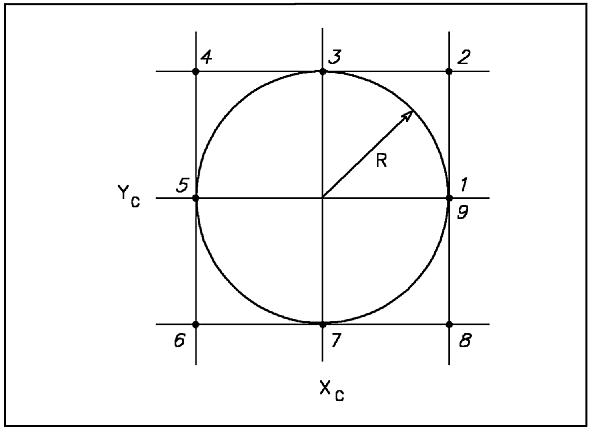
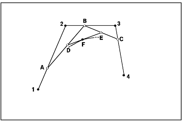
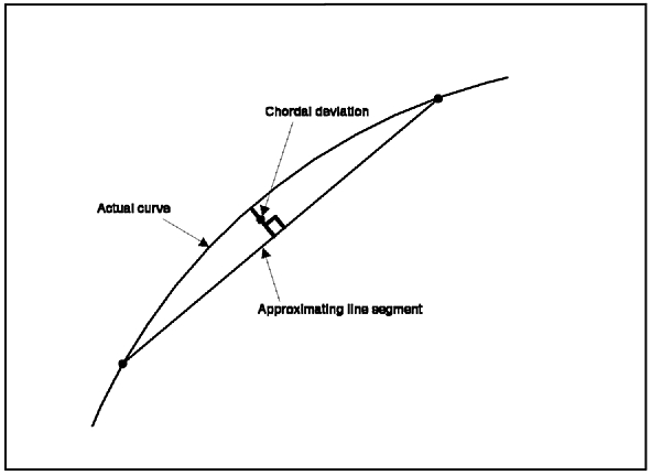
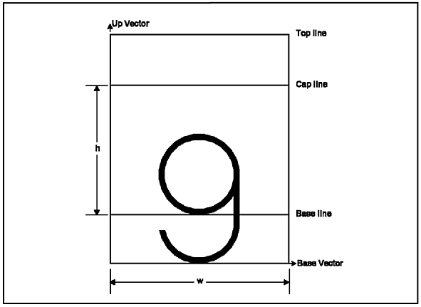
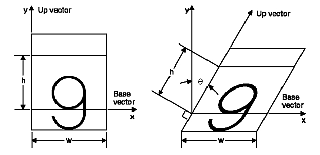
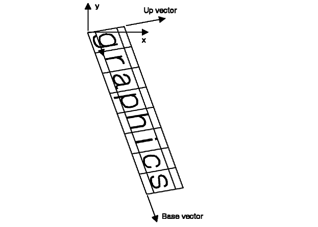
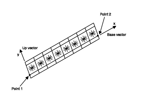
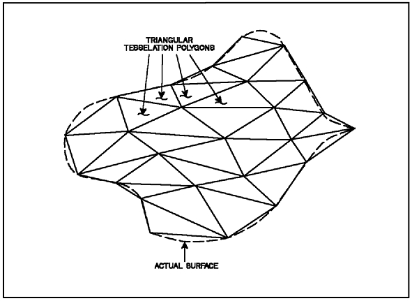