This chapter reviews the basic data elements that form structures. It presents output primitive elements such as lines, markers, polygons, and text. Along with a discussion of how to define each primitive, this chapter describes how to control their appearance through attribute settings and how to use modeling transformations to affect the size, shape, location, and orientation of primitives.
The appearance of graphical data is controlled through output primitive attributes. Color, interior style, line type, are some of these attributes. For example, in Chapter 3, the line type of the house in the sample program was defined using an attribute-setting subroutine.
This section provides a general discussion of output primitive attributes. Later on, there will be discussions of specific attributes associated with each primitive.
When a primitive subroutine or an attribute-setting subroutine is called, a structure element is created. The effect of the element on the graphical model is not seen immediately. The data to perform the requested operation is placed in the graPHIGS API storage area, but the effect of the element is seen only after the structure containing the element is processed and displayed. This processing of a structure at display time (called structure traversal) is discussed further in Chapter 6. "Displaying Structures"
The graPHIGS API provides two ways for your application to assign an attribute to an output primitive:
For your application to control where a primitive obtains its attributes, the graPHIGS API provides Attribute Source Flags (ASFs). ASFs can be thought of as switches within a structure that indicate whether the primitive obtains an attribute directly from a conceptual register or from an entry in a workstation bundle table.
Each workstation maintains internally a set of conceptual registers that contain the current values of each attribute at display time. Your application can set the ASF of each attribute at any location within a structure to
| 1=BUNDLED | |
| 2=INDIVIDUAL |
through the Attribute Source Flag Setting (GPASF) subroutine. Initially, all ASFs are set to INDIVIDUAL in order to obtain attributes directly from the conceptual attribute registers.
The system provides an ASF for each non-geometric primitive attribute. Some attributes, like geometric character height, are expressed in Modeling Coordinates (MC) and are affected when transformations are applied to the Modeling Coordinate System (MCS). Others, like color, have no effect on the output primitive orientation. The first type of attribute is a geometric attribute and cannot be included in a bundle table. The second is a non-geometric primitive attribute and can be bundled.
A special type of attributes that control detectability, highlighting, and visibility of all primitives are introduced in "Highlighting, Detectability, and Invisibility Class Specification"
The graPHIGS API provides attribute setting structure elements that enable your application to specify the value of each attribute individually. This method of attribute specification is workstation-independent. By using the proper structure elements, your application might change, for example, text color from red to green by specifying a color index.
In the Sample Program, the line type used to draw the house is 1=DASHED. This attribute is set by using the Set Linetype (GPLT) subroutine with a line type index of 2. Try changing this index to different values.
Internally, each workstation maintains a set of conceptual registers that contain the current values of each attribute during display traversal. The graPHIGS API lets your application change the conceptual attribute settings through attribute setting structure elements. When an output primitive is encountered during display traversal, the API uses the current values in the registers to draw that primitive.
When beginning the traversal of a structure, the conceptual attribute registers contain default values. If the application has defined no attributes, as is the case of the Sample Program, these default values are then used to display the graphical data. Also, in hierarchical structure networks, if the child structure has no attribute settings, the current values of the attributes (either default or defined by its parent structure) are used.
The graPHIGS API gives your application the ability to group attribute settings into tables of output primitive attributes called bundle tables Each workstation has its own bundle tables. This lets your application use a common index across workstations to specify attribute settings that are defined in workstation-dependent tables.
For each type of bundle table, there is a Set Representation subroutine call to set or change the bundle table contents. Please note that this subroutine call does not create a structure element.
The information in bundle tables exists independently of your application's graphics data. In order to establish a connection between an output primitive and an entry in the bundle table, your application specifies an index that points to that entry through a set bundle table index structure element.
Each output primitive uses one or more bundle tables. For example, polygons use the edge and interior bundle tables, while polylines use only the polyline bundle table.
Refer back to the modified Sample Program and modify it again as follows:
| Sample Program |
|---|
Refer to your house sample program and modify it as follows.
|
Recompile, load and run the program after making these modifications. The image displayed should be red with a solid line type.
Instead of defining the attributes individually, you are now using bundle table definitions. In the first statement of the DATA CREATION section, you have stored attribute settings in the first table index entry of the polyline bundle table of the workstation (GPXPLR) Then, in the structure, using the Attribute Source Flag Setting (GPASF) subroutine, you have set the line typ e, width and color of the polyline to BUNDLED. Use the Set Polyline Index (GPPLI) subroutine to set the attribute for the polyline.
By specifying attribute settings through table entries, your application can associate all of the values in a particular entry with an output primitive by simply specifying the index to that entry. This saves your application from redefining every attribute of commonly used output primitives. If your application sets the index such that it points beyond the last table entry, the system, during traversal, uses table entry 1.
Using an index to obtain attribute values has an additional value. You can set the bundle tables of different workstations such that the same index entry compensates for the workstation's differences. For example, line types can be used to differentiate between lines on a workstation with a monochrome display, and color can be used to do the same on a workstation with color display.
Bundling also provides a simple method of standardizing multiple instances of a model's appearance. For example, an application program modeling a bolt may put the structure in many locations. In each instance, the application program provides an index to a predefined entry in the polyline bundle table just prior to invoking the bolt structure.
The following table depicts a sample polyline bundle table.
Table 1. Sample Polyline Bundle Table
| Index | Linetype | Linewidth | Color Index |
|---|---|---|---|
| 1 | 1 | 1.00 | 2 |
| 2 | 2 | 0.50 | 8 |
| 3 | 2 | 2.00 | 5 |
| 4 | 1 | 1.50 | 3 |
| 5 | 3 | 1.00 | 4 |
| 6 | 1 | 1.00 | 9 |
| 7 | 1 | 1.00 | 10 |
For each attribute, the ASF specifies whether a primitive obtains an attribute directly from an individual setting or through an entry in a workstation bundle table. The graPHIGS API permits your application to change many ASFs at once by specifying multiple attributes and their corresponding ASF values in the same GPASF subroutine.
| Sample Program |
|---|
Refer back to the sample program as you have it after adding the previous modifications. Sample Program Do the following:
|
Recompile, load, and run the program after you have input these modifications. You will notice the house and door are no longer dashed; they now appear dotted.
You are using mixed attribute specifications. Your application has the ASF individual flag on for the line type (attribute identifier 1). Although the polyline bundle entry you have created specifies line type of 2=DASHED , due to the ASF flag setting for line type, the application obtains its line type attribute setting from the GPLT(3) subroutine call instead, which is set to 3=DOTTED
In the case of the sample program we are using one bundle table; the polyline bundle table. In the case of polygons, two bundle tables are used; the interior bundle table and the edge bundle table. For example, your application might use the GPASF subroutine to set the polygon output primitive's:
After using GPASF to set the edge line type and interior style to 1=BUNDLED , your application can specify which entry to use in the edge bundle table and interior bundle table using the Set Edge Index (GPEI) and Set Interior Index (GPII) subroutines respectively.
In the above example, the system obtains the edge line type from the edge bundle table and the interior style from the interior bundle table. The system ignores the color value entry from the interior bundle table and obtains it directly from its conceptual register, as specified by the interior color ASF.
Please note that if a parent structure exists, indexes to bundle table entries and individual (2=INDIVIDUAL ) settings are both inherited.
Because the graPHIGS API provides the tools necessary to develop workstation-independent programs, you may not need to change the attribute specifications in your application program to accommodate the differences between workstations. The graPHIGS API automatically maps workstation-independent attribute specifications to the closest workstation-dependent attribute specifications that can be realized at the target workstation. This section addresses the way in which workstation capabilities affect realized attribute values for scale factors and indexed tables.
At draw time, the system maps all application-specified, scale-factor attribute values to the closest scale factor value supported by the workstation. Then it multiplies that scale factor by the workstation's nominal value to obtain the primitive's size in Device Coordinates (DC). Your application can inquire the system defaults for these values. It can also inquire the workstation's supported values while the workstation is open.
The following table shows a case in which the workstation
supports four scale factor values (0.5, 1.0, 2.0, and 3.0)
with a nominal size of 2 Device Coordinates (DCs):
Table 2. Example of Workstation Support of Four
Scale Factor Values.
| Application-
Specified Scale Factor |
Closest Scale Factor
That is Available on This Device (DSF) |
Output Device
Nominal Size of Primitive (N) |
Size of
Primitive (DSF x N) |
|---|---|---|---|
| 1.0 | 1.0 | 2 | 2 |
| 0.2 | 0.5 | 2 | 1 |
| 0.7 | 0.5 | 2 | 1 |
| 1.5 | 2.0 | 2 | 4 |
| 7.0 | 3.0 | 2 | 6 |
Each workstation has its own bundle and color tables. In order to remain workstation-independent, your application uses indexes to specify entries into these tables. The workstation simply applies the specified index value to its own table. For example, the same workstation-independent index value that indicates blue on a color display can indicate a corresponding greyshade on a monochrome display.
The system provides default values for all workstation table entries when it opens the workstation. These defaults can be found in The graPHIGS Programming Interface: Technical Reference , or by using the appropriate inquire subroutines.
Colors in the graPHIGS API are assigned using tables of color specifications. A color table has entries that specify the values of the red, green and blue intensities defining a particular color. Each color table is workstation-dependent. A color is assigned to a primitive or a view by specifying an index into a workstation's color table.
The Set Color Representation (GPCR) subroutine can be used to load entries into the default workstation color table. The entries are loaded using the (GPCR) subroutine and are interpreted in the current workstation color model (discussed below). All workstations supported by the graPHIGS API have a default color model of RGB. Color table entries can be inquired using the Inquire Color Representation (GPQCR) subroutine. Notice that values returned by GPQCR are returned in the current workstation color model.
The graPHIGS API supports four methods for specifying color values. The four supported color models are:
The color model is a specification of a three-dimensional color coordinate system within which each displayable color is represented by a point. A workstation's color capabilities including whether color is supported, the default color model and the color palette size can be inquired using the Inquire Actual Color Facilities (GPQACF) subroutine. The current color model can be inquired using the Inquire Color Model (GPQCML) subroutine.
Each workstation has a preferred color model. For example, the IBM 5080 graphics system uses an RGB model. The initial table definition and subsequent entries are stored in this preferred model. If the application changes the current color model, all subsequent entries are converted from the new color model to the preferred model. Changes to the color model are not retroactive. In other words, all entries loaded before the color model change are not affected.
For each application defined color value, a workstation uses the available color which most closely matches the application defined values.
| Sample Program |
|---|
Look back at the previous version of the sample program Sample Program) and do the following.
|
Recompile, load and run the program after you have input these modifications. The color of the house is yellow, but now the door is brown.
By issuing the Set Color Representation (GPCR) subroutine, your application has redefined the color table of your workstation. Index six of your table now contains the color brown. Structure 2, the child structure, uses index six to set the color attribute of the door polyline. By setting its own color attribute, the child structure does not inherit its parent structure color setting. Try creating your own color table by specifying different values of red, green and blue intensities.
The graPHIGS API provides five basic output primitives that your application can use to define the parts of a graphics model. The graPHIGS API discusses advanced output primitives in Part Two of this book. Basic primitives include:
These output primitives and their attributes are discussed in the following sections.
Polylines provide a means for drawing lines of various types, widths, and colors. Drawing a polyline is like using a pen to draw a line on a piece of paper without lifting the pen from the page. If you need or want to break the line, you simply create a new polyline, or use the advanced disjoint polyline output primitive discussed in "Disjoint Polyline Primitive"
The polyline output primitive lets your application construct connected line segments in two or three dimensions.
For each polyline, your application provides a series of points in order to define its line segments. The graPHIGS API accepts, as input, one array into which your application has specified the X, Y, and Z modeling coordinate values for each point. The array is of a list of points that might look like: 1x,1y,1z,2x,2y,2z,...Nx,Ny,Nz.
The Polyline (GPPL2 and GPPL3) subroutines are used to create two- and three-dimensional polyline structure elements, respectively. At draw time, the system interprets the first X, Y, (and Z with the GPPL3 subroutine) coordinates as the starting point for the first line segment. The system then draws a line from the first coordinate point to the next coordinate point, then to the next, and the next, and so on.
With each of these subroutines, your application specifies:
The width parameter lets your application associate a variable number of array elements to each coordinate point. This allows application specific information to be included within the point list. The system ignores this information when constructing the polyline structure element.
Suppose your application uses the GPPL2 subroutine, and the array contains X, Y, Z, and T coordinates, where T can be the temperature at location (x,y,z), and the elements arranged 1x,1y,1z,1t,2x,2y,2z,2t,...Nx,Ny,Nz,Nt. This presents no problem. Your application specifies the number of points, a width of four, and the name of the array.
By specifying a width of four, your application knows that the interval between X coordinates is four array elements. By virtue of specifying a two-dimensional subroutine, such as GPPL2, the system automatically reads only the first two coordinates (X and Y values) in each interval. In a two-dimensional case such as this one, the effect of this width specification causes the system to skip the third and fourth elements of each interval. For all two-dimensional subroutine calls, the Z value automatically defaults to 0.
A two-dimensional specification is simply a shorthand way of specifying that Z=0. The system treats all graphics data as three-dimensional. (In reality, many devices will optimize on two-dimensional data. For the purposes of understanding how the graPHIGS API operates, you should think of 2D data as 3D with Z=0.).
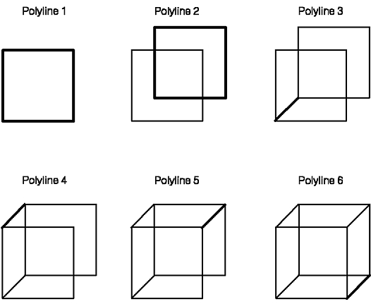
The figure, "Sample Polyline," depicts one way to use the polyline output primitive to construct the parts of a cube. At each stage, the application adds another polyline to the model. Each new polyline is highlighted by a bold line.
The sample program you have coded so far to draw the house uses the polyline output primitive. The following is a completely different program. It also uses the polyline output primitive and will display a star. The coordinates of the star are coded in the variable STAR the program is coded using the FORTRAN language and will use the 6090 workstation for display.
| Sample Program 2 |
|---|
Create this new sample program to learn how the graPHIGS API uses workstation default attribute values. * DECLARE VARIABLES
INTEGERx4 STATUS,CHOICE
INTEGERx4 WSID,STRID,VIEW1
REALx4 WINDOW(4),VIEWPT(4)
REALx4 STAR(12)
DATA WSID /1/
DATA STRID /1/
DATA VIEW1 /1/
DATA WINDOW /-10.0,10.0,-10.0,10.0/
DATA VIEWPT /0.0,1.0,0.0,1.0/
DATA STAR /-6.0,2.0,6.0,2.0,-4.0,-6.0,
* 0.0,6.0,4.0,-6.0,-6.0,2.0/
********************************************************************
* OPEN FUNCTIONS
CALL GPOPPH('SYSPRINT',0)
CALL GPCRWS(WSID,1,7,'IBM5080','5080 ',0)
********************************************************************
* VIEW DEFINITION
CALL GPXVR(WSID,VIEW1,14,VIEWPT)
CALL GPXVR(WSID,VIEW1,16,WINDOW)
CALL GPXVCH(WSID,VIEW1,1,8,2)
********************************************************************
* DATA CREATION
CALL GPOPST(STRID)
CALL GPPL2(6,2,STAR)
CALL GPCLST
********************************************************************
* DATA DISPLAY
CALL GPASSW(WSID,1)
CALL GPARV(WSID,VIEW1,STRID,1.0)
CALL GPUPWS(WSID,2)
********************************************************************
* INPUT FUNCTIONS
CALL GPRQCH(WSID,1,STATUS,CHOICE)
********************************************************************
* CLOSE FUNCTIONS
CALL GPCLWS(WSID)
CALL GPCLPH
STOP
END |
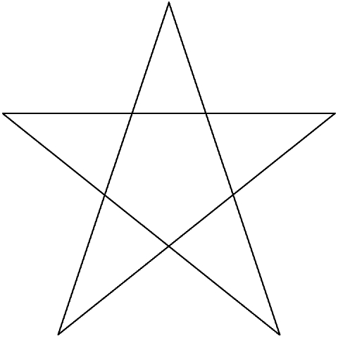
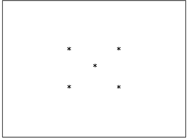
The figure, "Output from Star Sample Program," shows the graphic display you should get when you run the program:
Your drawing is a two-dimensional five point star. To draw a complete star the first and last coordinates must be the same. The total number of XY coordinates in the array is six. To display the star structure 1 contains only one element, a two-dimensional polyline structure element. No attribute elements are included in the structure, so the graPHIGS API uses workstation default attribute values. The star will appear white with solid lines.
The graPHIGS API lets your application control the attributes of the polyline output primitive from individual settings, a bundle table, or a mixture of both.
The individually set polyline attributes include:
The Set Linetype (GPLT) subroutine lets the application program specify an index into the workstation's line type table. The default line type table contains the following entries:
The Set Linewidth Scale Factor (GPLWSC) subroutine lets the application program specify how wide to make the polyline. The application program specifies the width as a fraction of the workstation's nominal linewidth. For example, a value of 2 yields a line twice as thick, within the capabilities of the device.
The Set Polyline Color Index (GPLCI) subroutine lets your application specify a color by providing an index value that points to an entry in a workstation's color table.
The Set Polyline End Type (GPPLET) subroutine controls the appearance of line ends. Line ends may either be flat (default), round or square. Flat ends are the default and are placed at the endpoints of lines. Round ends are semicircles centered at the line end, having a diameter equal to the linewidth. Square ends are identical to flat ends except they extend one half linewidth past the line's endpoint.
The API lets your application specify and use bundled polyline attributes.
The Set Extended Polyline Representation (GPXPLR) subroutine enables your application to load a polyline bundle entry, on a specified workstation, consisting of polyline line type, linewidth scale factor, and color values. These values are discussed above, individually.
Your application specifies which table entry to load through a parameter of the GPXPLR subroutine. This procedure is used to modify the workstation's polyline bundle table.
The Set Polyline Index (GPPLI) subroutine creates a structure element that points to an entry in the workstation's polyline bundle table. That entry contains a set of polyline attributes either set by the GPXPLR subroutine or set by default.
When encountering a polyline primitive at draw time, the system applies only those bundled attributes that are in effect at that time, as specified by the polyline ASFs.
| Modified Sample Program 2 |
|---|
Refer back to the star sample program. Sample Program Modify it according to the following:
|
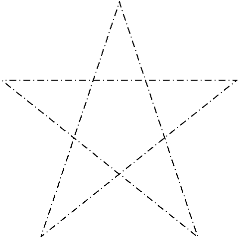
Recompile, load, and run the program after inputting these modifications. The figure, "Polyline Star with New Attributes," shows the image displayed.
The changes explained above will allow your application to use mixed attribute specifications. By using GPXPLR you have changed polyline bundle table index four. In the structure, the GPASF structure element specifies that only the line type and color attributes are bundled. Then, the GPPLI indicates the bundle table index for these attributes. The GPLWSC specifies the line width scale factor individual attribute. The star is drawn with red dashed lines.
Polymarkers give your application the ability to specify transformable point locations using various types, sizes, and colors of markers.
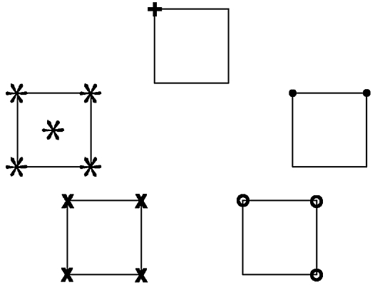
A single polymarker output primitive can mark several points. The figure, "Marker Type Illustrations," depicts various polymarker output primitives. The squares are not part of the polymarker output primitive, they are included in the drawing for explanation purposes only.
If you need to mark points, use the Polymarker (GPPM2 and GPPM3) subroutines. These subroutine calls create structure elements that are used to specify markers in either two- or three-dimensional Modeling Coordinate Systems (MCS).
As with the polyline and polygon primitives, your application provides a series of modeling coordinate points. Your application must declare a pointlist with X, Y, and optionally Z coordinates to locate the desired number of polymarkers.
Only the position of markers is fully transformable. In order to change a marker's size, the API provides a scale factor that operates independently of any scaling done to the model. So that the markers are always readable, the API does not perform rotational transformations on them.
The following program will help you understand the polymarker output primitive. The coordinates of the different locations where the polymarker will be displayed are coded in the variable POLYGN Compile, load and run the program. The program is coded in FORTRAN and uses the 5080 workstation for display.
| Sample Program 3 |
|---|
For a better understanding of polymarker output primitives, create the following program. * DECLARE VARIABLES
INTEGERx4 STATUS,CHOICE
INTEGERx4 WSID,STRID,VIEW1
REALx4 WINDOW(4),VIEWPT(4)
REALx4 MARKER(10)
DATA WSID /1/
DATA STRID /1/
DATA VIEW1 /1/
DATA WINDOW /-10.0,10.0,-10.0,10.0/
DATA VIEWPT /0.0,1.0,0.0,1.0/
DATA MARKER /0.0,0.0,-5.0,5.0,5.0,5.0,
* 5.0,-5.0,-5.0,-5.0/
********************************************************************
* OPEN FUNCTIONS
CALL GPOPPH('SYSPRINT',0)
CALL GPCRWS(WSID,1,7,'IBM5080','5080 ',0)
********************************************************************
* VIEW DEFINITION
CALL GPXVR(WSID,VIEW1,14,VIEWPT)
CALL GPXVR(WSID,VIEW1,16,WINDOW)
CALL GPXVCH(WSID,VIEW1,1,8,2)
********************************************************************
* DATA CREATION
CALL GPOPST(STRID)
CALL GPPM2(5,2,MARKER)
CALL GPCLST
********************************************************************
* DATA DISPLAY
CALL GPASSW(WSID,1)
CALL GPARV(WSID,VIEW1,STRID,1.0)
CALL GPUPWS(WSID,2)
********************************************************************
* INPUT FUNCTIONS
CALL GPRQCH(WSID,1,STATUS,CHOICE)
********************************************************************
* CLOSE FUNCTIONS
CALL GPCLWS(WSID)
CALL GPCLPH
STOP
END |
The figure, "Sample Program Output," shows the graphic display you will get when you run the program:
In the sample program you have just coded, structure 1 contains only one element, the two-dimensional polymarker output primitive. No attribute elements are included in the structure. To let you display your graphic model, the graPHIGS API will use the workstation default attribute values.
While the polymarker primitive positions a polymarker, polymarker attributes describe the appearance of the polymarker primitive. Your application can specify its attributes individually or by providing a bundle table index.
The individually set polymarker attributes include:
The Set Marker Type (GPMT) subroutine lets your application specify an index into the workstation's marker table. A workstation will support a subset of the following markers:
DOT                    (.)
PLUS SIGN              (+)
ASTERISK               (*)
CIRCLE                 (o)
DIAGONAL CROSS         (x)
The Set Marker Size Scale Factor (GPMSSC) subroutine lets your application specify the sizes of markers. Your application specifies a scale factor that is mapped to the closest supported workstation-defined scale factor value. Then, the system multiplies that scale factor value by the workstation's nominal size to determine the actual size of the polymarker on the output device. Your application can find the range of supported values in the WDT.
The Set Polymarker Color Index (GPPMCI) subroutine lets the application program specify the color of the marker. The application program supplies the GPPMCI with an index value that points to an entry in a workstation's color table.
The graPHIGS API lets your application modify and use bundles of polymarker attributes with the following subroutine calls:
The Set Extended Polymarker Representation (GPXPMR) subroutine enables your application to specify a bundle entry consisting of polymarker type, size, and color values. These values are discussed above, individually.
A parameter in the GPXPMR subroutine lets your application specify which entry in the workstation's polymarker bundle table to load. This procedure fills the workstation's polymarker bundle table. Notice that the GPPMR subroutine does not create a structure element, it only loads a table entry.
The Set Polymarker Index (GPPMI) subroutine creates a structure element that points to an entry in a workstation's polymarker bundle table. That entry contains a set of polymarker attributes either loaded by the GPPMR subroutine or set by default.
When encountering a polymarker primitive at draw time, the system applies only those bundled attributes that are in effect at that time, as specified by the polymarker ASFs.
| Modified Sample Program |
|---|
Refer back to the polymarker sample program you have coded. Sample Program Modify it now as follows:
|
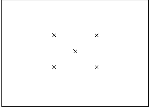
Recompile, load and run the program after you have input these modifications. The figure, "Sample Program Output," shows the image displayed.
By adding individual attribute specifications to the structure you have modified the appearance of the polymarker output primitive. The asterisk has been changed with the GPMT subroutine to a diagonal cross and its size has doubled. The color index refers to the workstation default color table in which index 2 is the color red.
Polygons let your application create closed bounded areas and control the appearance of their interiors and edges.
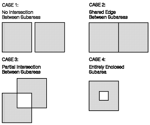
Your application can define a single polygon output primitive that has one or more closed bounded subareas. Notice that every subarea of a given polygon must be in the same plane. Subareas of the same polygon output primitive may appear unconnected, share a common edge or edges, overlap partially, or overlap entirely. The figure, "One Polygon With its Two Subareas Arranged in Four Different Ways," shows one polygon with its two subareas arranged in four different ways. It also shows how the graPHIGS API will fill the polygon if the subareas overlap.
The following program will help you understand the polygon output primitive. The program will display a square whose coordinates are coded in the variable Polygn Compile, load and run the program. As before, the program is coded in FORTRAN and uses the 5080 workstation for display.
| Sample Program |
|---|
Create the following program for a better understanding of polygon output primitives. * DECLARE VARIABLES
INTEGERx4 STATUS,CHOICE
INTEGERx4 WSID,STRID,VIEW1
REALx4 WINDOW(4),VIEWPT(4)
REALx4 POLYGN(8)
DATA WSID /1/
DATA STRID /1/
DATA VIEW1 /1/
DATA WINDOW /-10.0,10.0,-10.0,10.0/
DATA VIEWPT /0.0,1.0,0.0,1.0/
DATA POLYGN /2.0,2.0,2.0,6.0,
* 6.0,6.0,6.0,2.0/
********************************************************************
* OPEN FUNCTIONS
CALL GPOPPH('SYSPRINT',0)
CALL GPCRWS(WSID,1,7,'IBM5080','5080 ',0)
********************************************************************
* VIEW DEFINITION
CALL GPXVR(WSID,VIEW1,14,VIEWPT)
CALL GPXVR(WSID,VIEW1,16,WINDOW)
CALL GPXVCH(WSID,VIEW1,1,8,2)
********************************************************************
* DATA CREATION
CALL GPOPST(STRID)
CALL GPPG2(1,4,2,POLYGN)
CALL GPCLST
********************************************************************
* DATA DISPLAY
CALL GPASSW(WSID,1)
CALL GPARV(WSID,VIEW1,STRID,1.0)
CALL GPUPWS(WSID,2)
********************************************************************
* INPUT FUNCTIONS
CALL GPRQCH(WSID,1,STATUS,CHOICE)
********************************************************************
* CLOSE FUNCTIONS
CALL GPCLWS(WSID)
CALL GPCLPH
STOP
END
|
In the sample program you have just coded, the polygon contains only one close bounded subarea, the square. The structure has only one element, the two-dimensional polygon output primitive. No attribute elements are included in the structure. Workstation default attribute values will be used by the graPHIGS API to display the image. These default values specify a hollow polygon, edges flag on and color white.
Generating the edges for polygonal subareas is conceptually similar to generating polylines. If the specified list of points does not close the subarea, it will automatically be closed by the graPHIGS API To close a subarea, the graPHIGS API draws a line segment between the first and last points. The polygon primitive can then start the next subarea of that polygon at any location on the same plane.
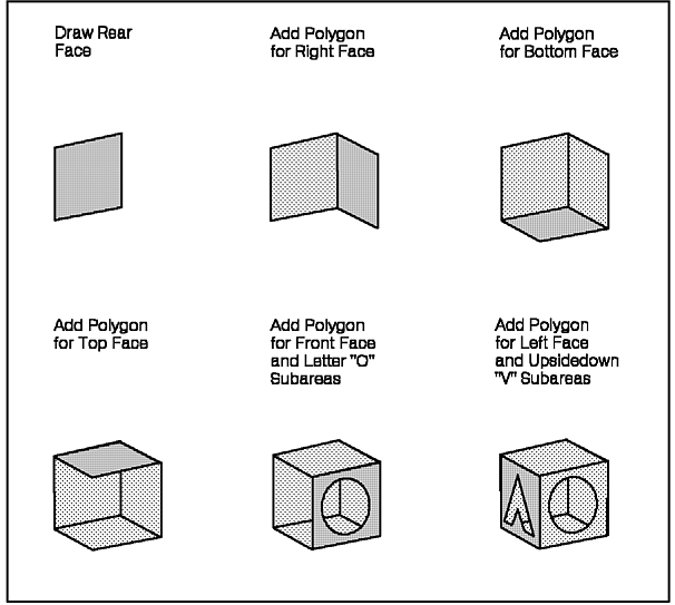
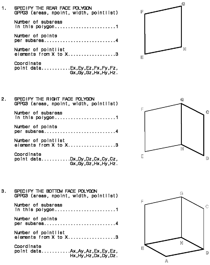
The figure, "Sample Polygon," is an example of one way to construct the parts of a cube. At each stage, the application adds another polygon to the model. The edge of each new polygon is highlighted by bold lines. Notice that the subarea forming the letter "O" is part of the same polygon as the front face of the cube. Likewise, the subarea forming the upside-down "V" is part of the same polygon as the left face of the cube.
The Polygon (GPPG2 and GPPG3) subroutines let your application create two- and three-dimensional polygon structure elements.
As with the polyline output primitive, your application must provide an array with the X, Y, and optionally Z values. Your application specifies the number of points in each subarea.
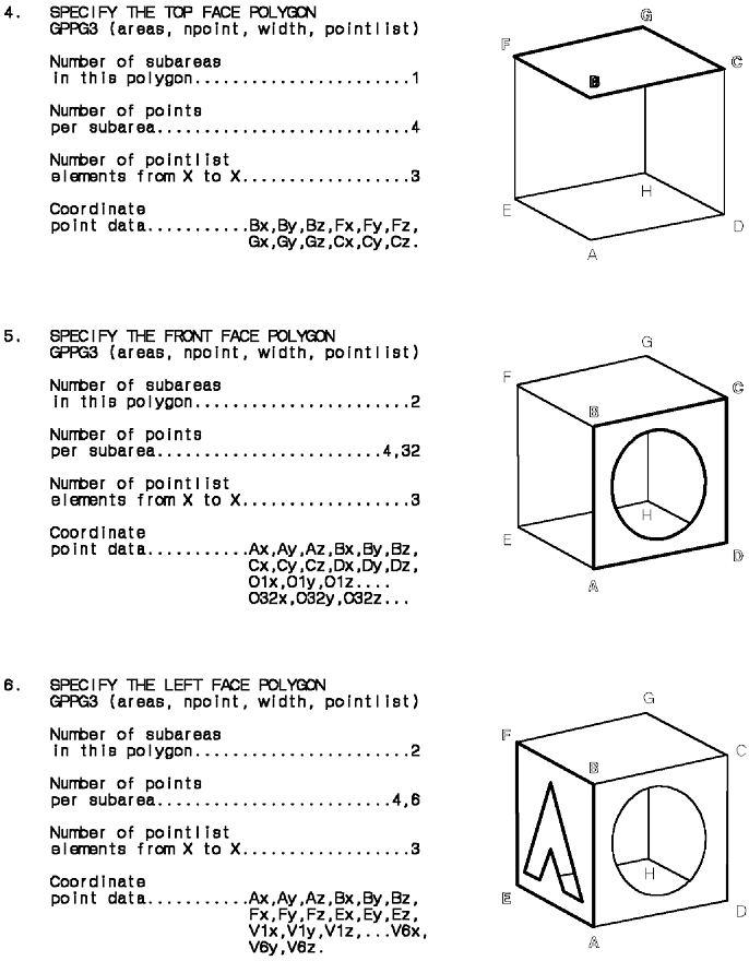
The figures, "One Way to Draw a Three-Dimensional cube (Part 1 of 2)" and "(Part 2 of 2)," depict the logical steps for drawing a three-dimensional cube with a sequence of GPPG3 output primitive subroutine calls. Notice that this is only one solution.
As shown in the figure, your application must apply the following:
Notes:
The graPHIGS API lets your application control the attributes of the polygon output primitive from individual settings, from a bundle table, or from a mixture of both.
The individually set polygon attributes include:
Edge FlagThe edge attributes are similar to the polyline attributes. The interior attributes apply to the interior areas of a polygon.
The Set Edge Flag (GPEF) subroutine creates a structure element that specifies whether or not the edge is drawn. A polygon edge is drawn on top of the interior's perimeter. If the application program sets the GPEF to 1=OFF the edge is not displayed, but the designated interior of the polygon is displayed. Notice that if the Interior Style is 1=HOLLOW and the edge flag is 1=OFF , the boundary is displayed in the color of the interior.
The Set Edge Linetype (GPELT) subroutine lets your application program specify one of the following line types for the polygon edges:
1=SOLID_LINE (system initialized value)For some workstations your application may specify additional line types.
The Set Edge Scale Factor (GPESC) subroutine lets your application specify how wide to make the polygon edges.
The Set Edge Color Index (GPECI) subroutine lets your application select a color for the polygon edge. The GPECI specifies an edge color by providing an index value that points to an entry in a workstation's color table.
The Set Interior Style (GPIS) subroutine lets your application specify whether the interior of a polygon is:
The Set Interior Color Index (GPICI) subroutine establishes the interior color of the designated polygon. GPICI specifies the color by providing an index value that points to a color in a workstation's color table.
The Set Interior Style Index (GPISI) subroutine lets your application specify an index to a pattern from the pattern table, or a hatch from the workstation-dependent hatch table, depending on the setting in the GPIS subroutine.
The polygon primitive obtains its attributes from two bundle tables. One for edges and another for interiors. Your application can specify and use bundles of edge and interior attributes with the following subroutine calls:
Set Edge RepresentationThe Set Extended Edge Representation (GPXER) subroutine enables your application to load a bundle entry consisting of edge flag, line type, scale factor, and color index values. These values are discussed above, individually. Your application specifies which entry in the workstation's edge bundle table to load, through the index parameter in the GPER subroutine.
The Set Edge Index (GPEI) subroutine creates a structure element that points to an entry in the workstation's edge bundle table. That entry contains a set of edge attributes either loaded by the GPER subroutine or set by default.
The Set Extended Interior Representation (GPXIR) subroutine enables your application to load a bundle entry consisting of interior style, color index, and style index values. These values are discussed above, individually. Your application specifies which entry in the workstation's interior bundle table to load, through the index parameter in the GPIR subroutine.
The Set Interior Index (GPII) subroutine creates a structure element that points to an entry in the workstation's interior bundle table. That entry contains a set of interior attributes either loaded by the GPIR subroutine or set by default.
When encountering a polygon primitive, at draw time, the system applies only those bundled attributes, if any, that are in effect at that time.
The graPHIGS API gives your application the ability to define its own interior fill pattern. The Set Pattern Representation (GPPAR) subroutine lets your application define a table entry that is used to create 2D grid of display color table indexes. Notice that the system overlays these patterns on the final orientation of the model. Use inquiries for device specific support information regarding interior fill patterns.
Geometric text gives your application the ability to define fully transformable text strings from system-provided, or user-supplied, text fonts. This section describes geometric text and its attributes.
If desired, the graPHIGS API lets your application define geometric text strings as part of a graphics model. In this case, the same transformations that affect the model also affect the text string. Naturally, the graPHIGS API also lets your application apply transformations to geometric text strings that are defined on their own and are independent of any model.
The Geometric Text (GPTX2 and GPTX3) subroutines let your application create a geometric text structure element in two- and three-dimensional Modeling Coordinates (MCs).
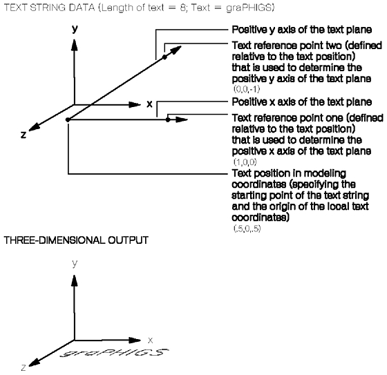
A three-dimensional text string implies that the text string called the text plane has a three-dimensional orientation. Your application defines the text plane by defining a text position and two reference vectors. The text position acts as the origin of the text string's local coordinate system.
The application program must provide data that specifies the text's:
Starting pointNote: The text plane's x-axis and text plane's y-axis are needed only for three-dimensional text specifications. The two-dimensional geometric text primitive uses the default values 1, 0, 0, to define the text plane's x-axis, and 0, 1, 0, to define the text plane's y-axis. This is the only difference between two- and three-dimensional text. Text specified as two-dimensional is fully transformable in three dimensions.
The figure, "Sample Text String Data and Its Three-Dimensional Output," depicts how the GPTX3 subroutine uses text string data to create three-dimensional text string output. In this example, the text string's xy plane equals the world coordinate system's xz plane.
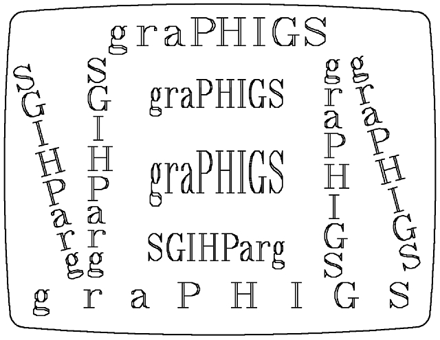
Geometric text attributes let your application control various aspects of the text. The figure, "Geometric Text Attributes," offers several ways in which geometric text attributes can alter the appearance of the geometric text.
Your application can control whether a geometric text string obtains all or part of its attributes individually or from its bundle table.
Note: Both geometric and annotation text attributes share the same bundle table.
Table 3. Sample Character Set and Font Support
Table
The individually set text attributes include:
Text Character SetNote:
- Collectively, these attributes define the perimeter of an imaginary rectangle around the text string, called the text extent rectangle. These points are discussed in detail later.
- These attributes orient the entire text extent rectangle, relative to the origin of the text's local coordinate system, on the text plane defined by the GPTX2 and GPTX3 subroutines. These points are discussed in detail later.
Character Sets, Fonts, and Colors: Character sets define a mapping used in text strings to map a binary code to a symbol shape. These can be, for example, national language alphabets or special technical symbols. The graPHIGS API supports a wide range of character sets representing the IBM supported national languages as well as user-defined character sets (refer to The GrapPHIGS Programming Interface: Technical Reference for details on user-defined character sets). The Set Text Character Set (GPTXCS) subroutine sets the current character set identifier (CSID) to the specified character set.
Notice that unlike other attributes, character sets are bound to text primitives when the primitive is defined (created). After issuing a (GPTXCS) subroutine, the specified character set remains in effect until your application changes it through another (GPTXCS) subroutine. To change the character set of a text string, you must respecify both the character set attribute and then the text primitive. The default CSID is U.S. English.
Each physical workstation has a preferred character set called its primary character set. An IBM 5080, for example, gives you the ability to customize your workstation's primary character set to one of seven national languages. If your application specifes an unrecognizable character set identifiier, the workstation uses the primary character set. Refer to The GrapPHIGS Programming Interface: Subroutine Reference or The GrapPHIGS Programming Interface: Technical Reference for valid character sets.
The Set Text Font (GPTXFO) subroutine creates a structure element that modifies the current text font. This produces variations in the appearance of the character set. Every workstation supports a text font numbered one in the primary character set. This font is used as the default in case your application references an unsupported character set, character font combination.
Consider a scenario along with Table 3, in which a workstation uses Swedish as its primary character set. Remember, for Swedish to be its primary character set, that workstation must provide a font number one. Suppose (1) that your application attempts to specify a CSID of German and a font of three. Since, in this hypothetical case, the workstation does not spport that font, the API next attempts (2) to use a csid of German and a font of one. When that attempt also fails, the API defaults (3) to font number one of the primary character set (in this case, Swedish).
Table 3. Sample Character Set and font support
Table.
| Fonts | Character Set Identifiers | ||
|---|---|---|---|
| French | Swedish | German | |
| 1 | X | X (3) | (2) |
| 2 | X | X | |
| 3 | X | X | (1) |
| 4 | X | X | |
| 5 | X | ||
| 6 | X | X | |
| 7 | X | X | |
The Set Text Color Index (GPTXCL) subroutine lets your application create a structure element that specifies the color index into the workstation's color table to be used when drawing the text. Your application supplies the GPTXCL with an index value that points to a color in the workstation's color table.
Character Box: The characters in any font are defined in their own local, two-dimensional, Cartesian coordinate system. This system was used by the font designer and consists of the font's topline, capline, halfline, baseline, bottomline, leftline, centerline, and rightline.
The topline, bottomline, leftline, and the rightline form the character body boundaries. Characters are defined within the character body boundaries. However, kerns on characters may exceed the right and left boundaries.
The font designer specified the exact position of each character in its character cell. In many cases, the top of a character corresponds to the capline, and its bottom corresponds to the baseline. Each side of any character should have enough space to insure normal spacing between characters in a text string, These guidelines help avoid unintentional vertical and horizontal overlapping.
Fonts ar either fixed size or proportionally sized. All characters within a fixed size font have hte same character body boundaries.
Vertical text alignment lines, such as the topline and the bottomline, are parallel to the x-axis of the font's coordinate system. Likewise, horizontal text alignment lines, such as the leftline and the rightline, are parallel to the y-axis of the font designer's coordinate system. Notice that the centerline bisects the body. Also, do not confuse the font's coordinate system with the text string's coordinate system.
In order to alter the size or shape of any character, you need to understand how the graPHIGS API defines them. The height of any character is the distance between the capline and the baseline. The nominal width of any character is the distance between the leftline and the rightline. A character's aspect ratio is its width divided by its height. Hence, the character's width may be specified as its aspect ratio multiplied by its height. The actual width equals the nominal multiplied by the expansion factor specified by your application.
The Text Extent Rectangle is an imaginary box around a text string that is indirectly determined by text attribute values. The Set Text Path (GPTXPT) subroutine creates a structure element that specifies which direction to add succeeding characters of a text string.
The Set Character Height (GPCHH) subroutine lets your application create a structure element that specifies the height of a character body in Modeling Coordinates (MC). The height is the distance between the baseline and the capline of the character body. The default value is 0.01. Since the aspect ratio remains constant, this subroutine call affects the character width as well as its height.
When the path is right or left, the height of the text extent rectangle equals the distance between the topline and the bottomline of the character bodies inthe text string. The left side of the rectangle equals the leftmost leftline of the character bodies in the text string. The right side of the rectabgle equals the rightmost rightline of the character bodies inthe text string.
When the path is up or down, the width to the text extent rectangle equals the horizontal distance between the boundaries formed by the leftmost leftline and the rightmost rightline of the character bodies in the text string. The top of the rectangle equals the maximum topline of the characters in the text string. The bottom of the rectangle equals the minimum bottomline of the characters in the text string.
The Set Character Spacing (GPCHSP) subroutine lets your application specify the amount of additional space between character bodies. Spacing is specified as a fraction of the height.
Specifying a value of zero results in no additional space between character bodies in the direction of the text path. This is the default.
Specifying a value of one creates a space between character bodies, in the direction of the text path, that is equal to the character's height.
Specifying a negative value can cause the character bodies to overlap, in the direction of the text path.
The Set Character Expansion Factor (GPCHXP) subroutine lets your application create a structure element that indirextly specifies the width of the charaacter bodies in a text string. The expansion factor is a deviation from the character's standard width-to-height ratio. The system multiplies this value by the width-to-height ratio to produce a new character width.
The default value (one), produces no deviation. specifying a value between zero and one reduces the width. Specifying a value greater than one increases the width. Values less than or equal to zero are invalid.
The Set Character Up Vector (GPCHUP) subroutine lets your application create a structure element that specifies what is considered "up" to the text string. It is specified as vector relative to the origin of the text string's local coordinate system.
Your application defines the up vector by specifying the direction of a vector in the text plane. The origin of the text plane is the origin of the up vector, and its direction is specified in the GPCHUP subroutine.
The Set Character Alignment (GPTXAL) subroutine lets your application use the parts of the character box to define the alignment of the entire text extent rectangle relative to the position.
Defining the alignment involves a pair of character box lines as applied to the text extent rectangle, one horizontal line, and one vertical line. The point where the two lines intersect determines the point on the text extent rectangle that corresponds to the text position. For example, your application may specify the intersection of the leftline and the baseline.
Though the GPTXAL subroutine uses character box lines, the system caluculates the alignment relative to the rectangle around the entire text string.
How the system applies the horizontal and vertical line specifications depends on the specified text path. The following figures depict the interdependences between text alignment and text path.
A leftline specification aligns the left side of the text extent rectangle with the text position. A rightline specification aligns the right side of the text extent rectangle with the text position. A centerline specification aligns the centerline of the entire text extent rectangle with the text position. A vertical line specification aligns the specified line, passing through all of the character bodies in the text string, with the text position.
A leftline specification aligns the left side of the text extent rectangle with the text position. A rightline specification aligns the right side of the text extent rectangle with the text position. A centerline specification aligns the centerline, the line midway between the rightline and the leftline of the text extent rectangle with the text position. A topline specification aligns the top of the text extent rectangle with the text position. A capline specification aligns the capline of the topmost character in the text extent rectangle, with the text position. A bottomline specification aligns the bottom of the text extent rectangle with the text position. A baseline specification aligns the baseline of the bottommost character in the text extent rectangle with the text position. A halfline specification aligns the halfline of the entire text extent rectangle with the text position.
Normal Alignment: In addition to the standard character body lines, the graPHIGS API lets your application specify a "normal" value (the default) for both the horizontal and vertical components of the pair. In order to achieve a natural alignment of characters that complements each text path, the system defines a normal specification as follows:
Text Precision: The Set Text Precision (GPTXPR) subroutine creates a structure element that controls how closely the system insures that the workstation's rendering of a text string corresponds to the defined appearance of that text srting. Each category identifies the minimum capabilities for that precision. A workstation may inplement more of the attributes than required for a given precision. For example, a workstation may implement character and stroke precision identically, as stroke precision. The following three kinds of text precision are supported:
Stroke precision causes the system to clip each vector of the text string exactly at the clipping volume boundaries.
Carefully choose a precision to meet the needs of your application. As you might expect, system overhead increases with increased precision. For example, you may need to consider that precision affects the rendering of a character's height when the text string is viewed in perspective. For stroke precision, perspective is applied to each vector in each character. For string precision, the character height to be used is determined by using the leading edge of the first character of the entire string.
Also, evaluate the trade-off between the need for exactness and performance. If your application does not demand precise renderings, you may opt for a precision that requires less system resources. Refer to the GPTXPR subroutine in The graPHIGS Programming Interface: Subroutine Reference for tables that describe the text precisions and their corresponding attributes.
The graPHIGS API specifies and uses bundles of text attributes with the following subroutine calls:
The Set Text Representation (GPTXR) subroutine enables your application to load a bundle entry consisting of text font, text color, character spacing, character expansion factor, and text precision values. These values are discussed above, individually. Other attributes that are affected by transformations are not bundled. In addition, the CSID is not bundled since it is a definition-time attribute.
Your application specifies which entry in the workstation's text bundle table to load, through a parameter in the GPTXR subroutine. The GPTXR subroutine does not create a structure elem ent. The Set Text Index (GPTXI) subroutine creates a structure element that points to an entry in the workstation's text bundle table. That entry contains a set of text attributes either loaded by the GPTXR subroutine or set by default. When encountering a text primitive, at draw time, the system applies only those bundled attributes, if any, that are in effect at that time as specified by the text ASFs.
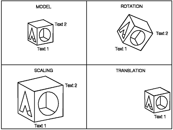
When you want to use text for menus or for annotating a part of a graphics model, use annotation text. Because the orientation and size of annotation text is not affected by rotation and scaling transformations, it provides better performance than geometric text, and is always readable.
Though each annotation text string is anchored to a transformable point, the text itself is not transformed. The text string is oriented so it is always readable to users, such as display screen operators. The figure, "How Annotation Text Readability is unaffected by Transformations," shows that various transformations do not affect the readability of annotation text.
The Annotation Text (GPAN2 and GPAN3) subroutines require your application to specify a location in the Modeling Coordinate System (MCS) from which your application positions the text. They also require your application to specify the number of characters in the text string and characters themselves.
The graPHIGS API lets your application control annotation text attributes individually and through bundle tables. The annotation text attributes are:
The Annotation Height Scale Factor is described here. The other annotation attributes are described in "Geometric Text" and Chapter 11. "Structure Elements"
Notes:
The Set Annotation Height Scale Factor (GPAHSC) subroutine enables your application to specify the height of annotation text. The system multiplies the Annotation Height Scale Factor by a device-dependent nominal character height and maps the result to the nearest character size supported by the output device.
All coordinate data in the graPHIGS API is conceptually manipulated as three-dimensional (3D) data. An application specifies a coordinate as an (XYZ) triplet. A two-dimensional (2D) coordinate is specified as an (XY) pair and is assumed to have Z=0. All points are then represented mathematically as row vectors:
point = ( X, Y, Z, W)
In this form, the point is represented as a homogeneous
coordinate, with W=1.
The graPHIGS API conceptually inserts the fourth coordinate value
and applications have no access to this W component.
As you will see, the W component
is necessary for applying transformations.
Transformations are represented as a 4 [default] 4 matrix as follows:
  |m11 m12 m13 m14|
  |m21 m22 m23 m24|
  |m31 m32 m33 m34|
  |m41 m42 m43 m44|
As with two-dimensional coordinate data, 2D transformation matrixes are conceptually expanded to 3D. This occurs as follows:
  |a b c|         |a b 0 c|
  |d e f| ----->  |d e 0 f|
  |g h i|         |0 0 1 0|
                  |g h 0 i|
At this point all coordinate data and transformation values are three-dimensional.
A transformation of coordinates is nothing more than a matrix multiplication. The transformation of a point, P, by the transformation matrix, M, may be represented as follows:
                |m11 m12 m13 m14|
                |m21 m22 m23 m24|
  [X Y Z 1]     |m31 m32 m33 m34|  = [XT YT ZT WT]
                |m41 m42 m43 m44|


     (P)              (M)          =          (PT)
Where the resultant transformed point, PT, is the matrix product of P and M, in that order.
The graPHIGS API provides a set of modeling transformation subroutine calls for controlling the size, shape, and location of primitives.
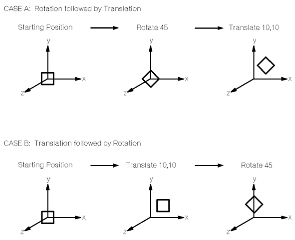
The order in which transformations are applied is significant. A translate preceding a scale or rotation around the origin yields results significantly different than a scale or rotation around the origin preceding a translation matrix. The figure, "Order Dependencies Between Translation and Rotation Around the Origin or Scaling," depicts some of the order dependencies between translation and rotation around the origin or scaling.
The modeling transformation that is used consists of a concatenation of two matrixes, a global transformation matrix and a local transformation matrix. The global transformation matrix is the inherited transformation matrix. However, the global transformation matrix can be reset by your application, using the Set Global Transformation (GPGLX3 and GPGLX2) subroutines. The current local transformation matrix represents a concatenation of all local modeling transformations in a structure prior to a primitive.
The Set Modeling Transformation (GPMLX2 and GPMLX3) subroutines provide a means of inserting a local modeling transformation matrix into a structure.
The graPHIGS API lets your application affect the order in which a modeling transformation matrix is concatenated with other local modeling transformations matrixes. The application can specify composition type:
These options can be useful in standardizing the placement of elements within structures. Suppose an application programmer begins each structure with a scale operation, followed by a rotate operation, followed by a translate operation. Without changing the order of the elements, the application program can specify that the translate operation precede the other transformations. To do this, the application program tells the system to preconcatenate the translation operation.
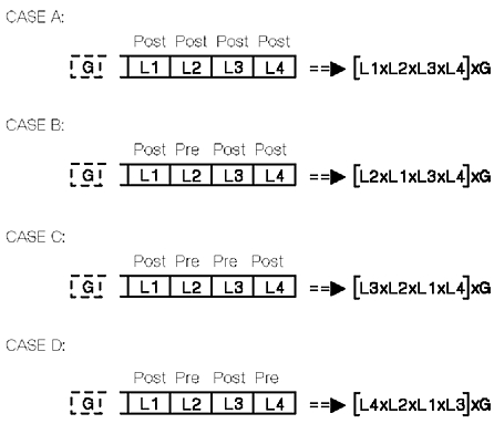
The figure, "Various Ways to Concatenate Matrixes," depicts various ways to concatenate matrixes. Notice that each element represented is a transformation, and that:
The graPHIGS API processes the set modeling transformation elements in the order they occur when all modeling transformations are designated as a postconcatenate type.
The graPHIGS API concatenates the set modeling transformation elements designated as a preconcatenate type before all preceding local transformations.
At the time when the graPHIGS API encounters a modeling transformation with the replace option specified, it replaces the current local modeling transformation.
Refer back to the house sample program. The following is how the DATA CREATION section should look:
. . .
       CALL GPOPST(STRID(1))
       CALL GPMLX2(MATRIX,POST)
       CALL GPASF(3,ATLIST,ATFLAG)
       CALL GPPLI(1)
       CALL GPPLCI(5)
       CALL GPPL2(6,2,HOUSE)
       CALL GPEXST(STRID(2))
       CALL GPCLST
*
       CALL GPOPST(STRID(2))
       CALL GPMLX2(TRANSD,POST)
       CALL GPPLCI(6)
       CALL GPPL2(5,2,DOOR)
       CALL GPCLST
.
.
.
The house sample program model has a parent structure (STRID (1)) that draws the house and a child structure (STRID The parent structure has a modeling transformation (MATRIX ) and the child structure has a modeling transformation (TRANSD ).
The modeling transformation (MATRIX ) allows the application to translate the house to the center of the screen. The concatenation of the global transformation (MATRIX ), inherited from the parent structure with the local modeling transformation (TRANSD ), translates the door to a position inside the house.
| Modified Sample Program 1 |
|---|
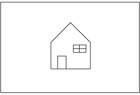
Now you will add a window to the house. You will use a polyline to draw the window. The coordinates of the window are defined in the variables: HWNDW1 , HWNDW2 and HWNDW3 Modify the program as follows.
|
Recompile, load and run the program after inputting these modifications. The figure, "House with Window," shows the image displayed.
You have added a blue window to the house. The window is a child structure of the house structure. It has a modeling transformation (TRANSW ). The concatenation of the global modeling transformation (MATRIX ), inherited from the parent structure, with the local modeling transformation (TRANSW ), translates the window to a position in the house on the center of the screen.
The Insert Application Data (GPINAD) subroutine creates a structure element that serves as a storage facility within a structure. For example, your application can use the GPINAD subroutine to insert arbitrarily complex comments within a structure. Application data inserted into structure elements can be retrieved using the Inquire Element Data (GPQED) subroutine.
The graPHIGS API lets your application group primitives into application-defined classes. The set of classes a primitive belongs to during display is an attribute of the primitive. This section shows you how to group primitives into attribute classes that let your application control the detectability, highlighting, and invisibility of primitives. Later, in "Resolving Detectability, Highlighting, and Invisibility" you learn how filters give your application control over which classes are detectable, highlighted, and invisible without needing to edit structures.
The Add Class Name to Set (GPADCN) subroutine creates a structure element that enables your application to include a primitive in a class.
All primitives that follow a GPADCN subroutine in a structure or sub-structure become members of the same class, unless the class is removed by the Remove Class Name from Set (GPRCN) subroutine. Primitives that follow the GPRCN subroutine are not i n the same class as primitives prior to the GPRCN subroutine.
Adding a new class does not cancel the effect of previously defined classes. In this case, succeeding primitives become members of both classes. The effects of the GPADCN subroutine are inherited.
The graPHIGS API provides an attribute setting that lets your application set the color to be used for highlighting primitives. The Set Highlighting Color Index (GPHLCI) subroutine lets your application specify an index into the color table. The default highlighting color index is one. When encountered at draw time, this element modifies the current highlighting color index.
When a primitive is highlighted, it is drawn using the
highlighting color rather than the color attribute of the
primitive.
For pixel primitives, a "boundary" (solid line) is
drawn around the pixel array using the highlighting color.
When a polygon is highlighted, the highlighting technique
depends on the edge flag and interior style settings (refer
to
"Polyline Attributes").
The effect of these settings on the displayed polygon is
detailed in the following table:
Table 4. Effect of Edge Flag and Interior Style
Settings on Polygon Highlighting
| Interior
Style Setting |
Edge Flag
Setting |
Polygon Highlighting Results |
|---|---|---|
| EMPTY | ON | The polygon edge is drawn using the highlighting color |
| EMPTY | OFF | A boundary (solid line) is drawn using the highlighting color |
| HOLLOW | ON | The polygon edge is drawn using the highlighting color |
| HOLLOW | OFF | A boundary (solid line) is drawn using the highlighting color |
| SOLID | ON | The polygon interior and edge are drawn using the highlighting color |
| SOLID | OFF | The polygon interior is drawn using the highlighting color |
| PATTERN | ON | The polygon edge is drawn using the highlighting color |
| PATTERN | OFF | A boundary (solid line) is drawn using the highlighting color |
| HATCH | ON | The polygon interior and edge are drawn using the highlighting color |
| HATCH | OFF | The polygon interior is drawn using the highlighting color |
The graPHIGS API provides an output primitive attribute that lets your application identify a primitive or group of primitives by name. The Set Pick Identifier (GPPKID) subroutine creates a structure element that modifies the pick identifier for subsequent primitives.