Chapter 16. Rendering Pipeline

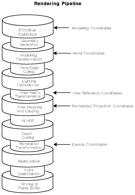
This chapter provides an overview of the graPHIGS API processing performed on primitives in order to generate output on a display surface. The sequence of processes applied to primitives in a graphics package is called its rendering pipeline. The figure, "The graPHIGS API Rendering Pipeline," shows each step in the graPHIGS API rendering pipeline process. This chapter explains the basic operation performed by each of these steps.

Following is a brief definition of each of the rendering steps. The advanced rendering concepts are discussed in detail in the remainder of this chapter and the next.

Primitive Definition

Geometric primitives are defined when your application creates primitive structure elements, such as polylines, polygons, NURBS curves and surface. Primitive definition is discussed in detail in the Chapter 4. "Structure Elements" and Chapter 11. "Structure Elements"

Morphing

Modifies the geometry and/or data (texture) mapping data of a primitive.

Geometry Generation

From a given primitive definition, a set of geometric entities are generated. The types of entities that are generated and their characteristics are determined by the geometric attributes of the primitive. For some entities, such as curves and surfaces, this step may be deferred to later in the pipeline after transformations have been performed on control points. This is done only if no distortion to lighting calculation is introduced by the transformation.

Modeling Transformation

Transforms the geometric entities by the matrix resulting from the concatenation of the current local and global modeling transformation matrixes.

Modeling Clipping

Provides a way to clip geometric entities in world coordinates.

Face/Edge Culling

Determines whether a given geometry should be further processed or not based on its geometric information. In most cases, the geometry examined in this step will be the normals of planar surfaces. This step can, for example, reject a primitive based on its normal.

Lighting Calculations

Simulates the effects of light sources illuminating the primitives. This process is performed only on area geometries.

Data (Texture) Mapping

Uses data values from the vertices of primitives to determine the colors to be used to render the primitives. Texture Mapping is a method of filling the interior of area primitives from a collection of colors.

View Matrix Transformation

Transforms the resulting geometry to view reference coordinates by using the current view orientation matrix.

View Mapping and Clipping

Performs the window to viewport mapping and perspective projection if specified. Primitives are also clipped to the view volume.

Hidden Line / Hidden Surface Removal (HLHSR)

Determines the geometric relationship between geometries within the scene. Based on the relation, it is decided whether a given geometry should be further processed or not.

Depth Cueing

Changes the color of geometries based on their z-location within Normalized Projection Coordinate (NPC) space. This helps give the generated picture an illusion of depth.

Workstation Transformation

Transforms the geometry of the primitive to device coordinates after being clipped to the workstation window.

Rasterization

Determines final shape of a given geometry by using its rendering attributes, such as line style, etc. The geometric shape is digitized to a set of pixel coordinates.

Transparency

Allows you to control the degree to which you can "see through" a primitive.

Color Quantization

Maps colors generated by the previous stages to those available on the workstation based on application specified controls. For detailed information on color quantization, see Chapter 17. "Manipulating Color and Frame Buffers"

Writing to Frame Buffer

Places the rendered output into the frame buffer,   possibly using a frame buffer operation and/or a masking operation. For detailed information on frame buffer operations, see Chapter 17. "Manipulating Color and Frame Buffers"

Morphing

Overview

Morphing lets you transform an object from one shape to another where the start and end shapes have the same number of vertices. The term itself is derived from the words metamorphosis or metamorphose, which mean changed or to change in form. You define the changes using morphing values at each vertex of the affected primitives along with scale factors that define how the vertex morphing values affect the primitive.

There are two types of morphing, one using vertex coordinates and the other using data mapping data values. These functions are called vertex morphing and data morphing, respectively.

You can use vertex morphing with the following primitives:

• Polyline Set 3 with Data (GPPLD3)
• Polygon 2 with Data (GPPGD2)
• Polygon 3 with Data (GPPGD3)
• Triangle Strip 3 (GPTS3)
• Quadrilateral Mesh 3 (GPQM3)

You can use data morphing with the following primitives:

• Polygon 2 with Data (GPPGD2)
• Polygon 3 with Data (GPPGD3)
• Triangle Strip 3 (GPTS3)
• Quadrilateral Mesh 3 (GPQM3)

Because data morphing applies to area primitives only, data morphing cannot be used for polylines.

Note: Use the Inquire Workstation Description (GPQWDT) call to determine whether your workstation supports the graPHIGS API morphing facilities.

Vertex Morphing

Vertex morphing allows you to modify the rendered geometry of the primitive without changing the structure element. To achieve the effects of morphing, your application must provide morphing vectors with each vertex in the primitive definition. These act together with the morphing scale factors to modify the rendered primitive. You use the Set Vertex Morphing Factors (GPVMF) subroutine to specify the scale factors. Vertex morphing vectors and scale factors affect only the vertex coordinates, while data morphing vectors and scale factors affect only the data mapping data values at each vertex.

Vertex morphing takes place in modeling coordinates. The modeling coordinate values specified in the primitives are modified by the vertex morphing process to produce new modeling coordinate values. These modified coordinate values are then used in the graPHIGS API pipeline processing to render the primitive. The values are used only during traversal and do not update any element content.

• Polygons: Polygon primitives are planar primitives, and the rendering results are undefined if all the points do not lie in the same plane. With vertex morphing you could cause polygons that are defined as planar in Modeling Coordinates to become non-planar (after the addition of the vertex morphing terms). To avoid undesirable rendering results when using vertex morphing with polygon and quadrilateral mesh primitives, your application should ensure that all vertex morphing operations result in planar polygons, or that all affected polygons define only triangles which by definition are always planar.
• Normal Vectors: Normals and other vertex values remain unchanged even if you modify the vertex coordinates through vertex morphing. If you specify normals with a primitive, they will be used as specified regardless of the change in geometry. This could cause unexpected lighting results. However, if you do not specify normals with a primitive and lighting is enabled, graPHIGS API automatically calculates a geometric normal for each primitive facet. (See "Geometry Generation" These normals are calculated after morphing, and reflect the modified geometry.

Data Morphing

Data morphing occurs in data space and results in morphed data values. That is, data morphing occurs before all transformations are applied to the data values in the graPHIGS API rendering pipeline. You use the Set Data Morphing Factors (GPDMF) subroutine to specify the data morphing scale factors.

Data morphing changes the vertex data mapping values, before the data matrix is applied. See Set Data Matrix 2 (GPDM2) and Set Back Data Matrix 2 (GPBDM2) procedures in The graPHIGS Programming Interface Subroutine Reference for more information on the data matrix specification. You can only specify Data morphing values if corresponding data mapping data values exist in the primitive definition.

Data morphing can be interpreted in different ways, depending on the data mapping method being used. See "Texture/Data Mapping" If you use data mapping for contouring to represent application-specific values such as temperature, then data morphing reflects temperature changes that may change the interior color of the primitive. If data mapping is used for texture mapping, then data morphing provides a means to stretch the texture image across the primitive.

The Morphing Equation

In vertex morphing, the vertex coordinate values (x, y, z) combine with the vertex morphing scale factors (s₁ , s₂ , ..., s_nscale) and the vertex morphing vectors ((dx₁ , dy₁ , dz₁ ), (dx₂ , dy₂ , dz₂ ), ..., (dx_nvector, dy_nvector, dz_nvector)) to create the new vertex coordinate values (x´, y´, z´) as follows:

x´ = s₁ x + s₂ dx₁ + s₃ dx₂ +...+ s_nscale dx_nvector

y´ = s₁ y + s₂ dy₁ + s₃ dy₂ +...+ s_nscale dy_nvector

z´ = s₁ z + s₂ dz₁ + s₃ dz₂ +...+ s_nscale dz_nvector

In data morphing, the data mapping data values (x₁ , x₂ , ..., x_ndata) combine with data morphing scale factors (s₁ , s₂ , ..., s_nscale) and data morphing vectors ((d_1,1 , _1,2 , ..., d_1,ndata ), (d_2,1 , _2,2 , ..., d_2,ndata ), ..., (d_nvector,1 , d_nvector,2 , ..., d_{nvector,ndata} )) to create the new data mapping data values (x´₁ , x´₂ , ..., x´_ndata ). This combination is of the form:

x´₁ = s₁ x₁ + s₂ d_1,1 + s₃ d_2,1 +...+ s_nscale d_nvector,1

x´₂ = s₁ x₂ + s₂ d_1,2 + s₃ d_2,2 +...+ s_nscale d_nvector,2

...

x´_ndata = s₁ x_ndata + s₂ d_1,ndata + s₃ d_2,ndata +...+ s_nscale d_{nvector,ndata}

Number of Scale Factors: These equations show that the number of morphing scale factors should be one more than the number of morphing vectors in the affected primitive (nscale = nvector + 1) if the number of morphing vectors and scale factors disagree at traversal time, then zero-value vectors or scale factors are assumed wherever necessary. That is, if you supply too many scale factors for a given primitive (nscale > nvector + 1), then the graPHIGS API ignores the extra scale factors as if there were additional zero-valued morphing vectors in the primitive definition. And, if too few scale factors are supplied (nscale < nvector + 1), the extra morphing vectors are ignored, as if there were additional scale factors supplied with value 0.

Scale Factor Constants: You supply data morphing scale factors as a list of parameters using Set Data Morphing Factors (GPDMF) and Set Back Data Morphing Factors (GPBDMF) subroutines.

You supply vertex morphing scale factors as a list of parameters using the Set Vertex Morphing Factors (GPVMF) subroutines.

You can query the maximum number of morphing vectors (and parameters) a particular workstation supports by using the Inquire Workstation Description (GPQWDT) subroutine.

Morphing Examples

You can use morphing to perform several different types of modifications to the rendered primitive values. This section contains a few examples.

Metamorphosis - Linear over Time

Morphing transforms one object's geometry into another, provided the same number of vertices are used to define both objects. The metamorphosis outlined in this section causes each vertex in the initial object to follow a linear path to the corresponding vertex in the final object.

1. Specify both object locations with each vertex. Let (x_initial, y_initial, z_initial) represent the location of a vertex at the initial time (t_initial), and (x_final, y_final, z_final) represent the same vertex at the final time (t_final). Then set the vertex coordinates and a single vertex morphing value:

   (x, y, z) = (x_initial, y_initial, z_initial)

   (dx₁ , dy₁ , dz₁ ) = (x_final, y_final, z_final)

2. For each time (t) between the initial and final times (t_initial <= t <= t_final), define u to represent the normalized time (0.0 <= u <= 1.0):

          (t - t

   _initial ) u = ------------------      (t_final - t_initial)

   Then set the vertex morphing factors:

   (s₁ , s₂ ) = ((1 - u), u)

   so that:

   (s₁ , s₂ ) = (1.0, 0.0) at time t_initial

   (s₁ , s₂ ) = (0.0, 1.0) at time t_final

Metamorphosis - Second Order Curve over Time

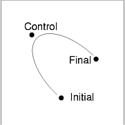
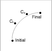
The metamorphosis outlined in this section causes each vertex in the initial object to follow the path of a second order Bezier curve to the corresponding vertex in the final object.

1. Specify both object locations and an additional control point with each vertex. Let (x_initial, y_initial, z_initial) represent the location of a vertex at the initial time (t_initial ), (x_final, y_final, z_final) represent the same vertex at the final time (t_final), and (x_control, y_control, z_control) represent the vertex control point. Then set the vertex coordinates and two vertex morphing vectors:

   (x, y, z) = (x_initial, y_initial, z_initial)

   (dx₁ , dy₁ , dz₁ ) = (x_control, y_control, z_control)

   (dx₂ , dy₂ , dz₂ ) = (x_final, y_final, z_final)

2. For each time (t) between the initial and final times (t_initial <= t <= t_final ), define u to represent the normalized time (0.0 <= u <= 1.0):

          (t - t

   _initial ) u = ------------------      (t_final - t_initial)

   Then set the vertex morphing factors:

   (s₁ , s₂ , s₃ ) = ((1 - u)² , 2u(1 - u), u² )

   so that:

   (s₁ , s₂ , s₃ ) = (1.0, 0.0, 0.0) at time t_initial

   (s₁ , s₂ , s₃ ) = (0.0, 0.0, 1.0) at time t_final

   Substituting these values in the vertex morphing equations, you see that (x, y, z) = (x_initial , y_initial , z_initial ) at time t_initial , and (x, y, z) = (x_final , y_final , z_final ) at time t_final, as shown in the figure, "Second Order Bezier Curve Over Time."

Metamorphosis - Third Order Curve over Time

The metamorphosis outlined in this section causes each vertex in the initial object to follow the path of a third order Bezier curve to the corresponding vertex in the final object.

1. Specify both object locations and two additional control points with each vertex. Let (x_initial, y_initial, z_initial) represent the location of a vertex at the initial time (t_initial), (x_final, y_final, z_final) represent the same vertex at the final time (t_final), and (x_c1 , y_c1 , z_c1 ) and (x_c2 , y_c2 , z_c2 ) represent the two control points. Then set the vertex coordinates and three vertex morphing vectors:

   (x, y, z) = (x_initial, y_initial, z_initial)

   (dx₁ , dy₁ , dz₁ ) = (x_c1 , y_c1 , z_c1 )

   (dx₂ , dy₂ , dz₂ ) = (x_c2 , y_c2 , z_c2 )

   (dx₃ , dy₃ , dz₃ ) = (x_final, y_final, z_final)

2. For each time (t) between the initial and final times (t_initial <= t <= t_final), define u to represent the normalized time (0.0 <= u <= 1.0):

          (t - t

   _initial ) u = ------------------      (t_final - t_initial)

   Then set the vertex morphing factors:

   (s₁ , s₂ , s₃ , s₄ ) = ((1 - u)³ , 3u(1 - u)² , 3u² (1 - u), u³ )

   so that:

   (s₁ , s₂ , s₃ , s₄ ) = (1.0, 0.0, 0.0, 0.0) at time t_initial

   (s₁ , s₂ , s₃ , s₄ ) = (0.0, 0.0, 0.0, 1.0) at time t_final

   Substituting these values in the vertex morphing equations, you see that (x, y, z) = (x_initial, y_initial, z_initial) at time t_initial, and (x, y, z) = (x_final, y_final, z_final) at time t_final, as shown in the figure, "Third Order Bezier Curve Over Time."

Data Contour Modification

Morphing also provides a means to represent changes in application-specific data, which causes variations in a primitive's   data mapping contour bands the contouring changes outlined in this section allow a single data value, namely temperature, to vary from one set of readings to another. These temperature changes are linear over time; however, non-linear data changes may also be accomplished in a manner similar to the vertex morphing examples above.

1. Specify both temperature readings with each vertex. Let temperature_initial represent the temperature of a vertex at the initial time (t_initial), and temperature_final represent its temperature at the final time (t_final). Then set the vertex data mapping value and one data morphing vector:

   x₁ = temperature_initial

   d₁ = temperature_final

2. For each time (t) between the initial and final times (t_initial <= t <= t_final), define u to represent the normalized time (0.0 <= u <= 1.0):

          (t - t

   _initial ) u = ------------------      (t_final - t_initial)

   Then set the data morphing factors:

   (s₁ , s₂ ) = ((1 - u), u)

   so that:

   (s₁ , s₂ ) = (1.0, 0.0) at time t_initial

   (s₁ , s₂ ) = (0.0, 1.0) at time t_final

Substituting these values in the data morphing equations, you see that x₁ = temperature_initial at time t_initial, and x₁ = temperature_final at time t_final.

Geometry Generation

The graPHIGS API includes many functions to process primitives based on their geometric data. In other words, assume that all geometric data is conceptually treated as one of the following:

1. Glyph

   This geometric entity is mathematically a point and so it has no spatial measure. However on the actual display surface, it is displayed as a set of pixels with a fixed relationship. Therefore on most workstations, it is treated as a planar object on a plane parallel to the display surface. This geometry is generated by the following primitives. Note that many of the listed primitives may generate more than one glyph.

   Polymarker 2/3
   Marker Grid 2/3
   Annotation Text 2/3
   Annotation Text Relative 2/3
   Pixel 2/3

2. Line

   A straight line connecting two endpoints. Like the glyph, it has no spatial measure but is displayed as a set of pixels approximating the mathematical line. Therefore, on most workstations it is treated as a planar object on a plane which includes the mathematical line. The plane will be a plane parallel to the display when the line itself is parallel to the display. Otherwise, the plane is a plane which intersects with the display surface on a horizontal or vertical line. This geometry is generated from the following primitives:

   Polyline 2/3
   Disjoint Polyline 2/3
   Polyline Set 3 With Data
   Polyhedron Edge
   Line Grid 2/3
   Circle 2
   Circular Arc 2
   Ellipse 2/3
   Elliptical Arc 2/3
   Non-Uniform B-Spline Curve 2/3

   and by the following primitives when they have the edge flag attribute on:

   Polygon 2/3
   Polygon With Data 2/3
   Composite Fill Area 2
   Triangle Strip 3
   Quadrilateral Mesh 3
   Non-Uniform B-Spline Surface
   Trimmed Non-Uniform B-Spline Surface

   For the quadrilateral mesh or the polygon with data primitive, the application can individually control whether a given edge generates a line entity or not by the boundary flags in the primitive definition.

3. Area

   A semi planar region surrounded by a closed sequence of lines. The term "semi" means that the region may not be exactly planar in some cases but is treated as planar. This geometric entity is generated by the following primitives:

   Polygon 2/3
   Polygon With Data 2/3
   Composite Fill Area 2
   Quadrilateral Mesh 3
   Triangle Strip 3
   Non-Uniform B-Spline Surface
   Trimmed Non-Uniform B-Spline Surface

4. Text

   A set of co-planar geometries which represent a sequence of character shapes. On some workstations, these geometries may be processed as if they are line or area geometries. Geometries of this category are generated only by the following primitives:

   Text 2/3
   Character Line 2

Geometric Attributes

Each primitive has many attributes. Some of them are used to generate geometric entities described in the previous section and affect the geometric processing described in this chapter. Others are bound to the entities and will be used for purposes other than geometric processing. We call attributes in the first group geometric attributes.

As described in the previous section, geometric entities generated by a given primitive may be different for each workstation. Therefore, a set of geometric attributes may also be workstation-dependent. For example, on a workstation which treats a line geometry as a planar object with some width, the line width scale factor attribute may affect the geometric processing and so it may be considered to be a geometric attribute.

To minimize such workstation dependencies, we define a set of attributes which are always treated as geometric attributes and another set of attributes which may be treated as geometric attributes or not depending on the workstation. Any workstation supported by the graPHIGS API products will never use other attributes as geometric attributes and so they will not affect the geometric processing described here.

Table 7. Workstation-dependent geometric attributes.

Curve Tessellation

On some workstations curves are divided into sets of line geometries before they are processed by the rendering pipeline. Such a process is called curve tessellation The application can control the process by the curve approximation criteria attribute in conjunction with its associated approximation value and possibly the tessellation vector specified in a curve definition itself.

The curve approximation criteria are defined in Chapter 11. "Structure Elements"

Note: The curve approximation criteria attribute is applied to the non-uniform curve primitives but is not applied to the circle, ellipse and arcs.

Surface Tessellation

As with curves, your application can control the tessellation of surfaces using the Set Surface Approximation Criteria attribute. The Set Surface Approximation Criteria (GPSAC) structure element defines two approximation values, one for the u and one for the v directions of the surface. The meaning of the approximation values are conceptually the same for curves and surfaces.

From the definition of the surface approximation criteria, a surface is tessellated into a set of area geometries each of which has a rectangular shape in the topological sense. However, a workstation may further divide the rectangle into a set of smaller pieces, typically into two triangles.

In addition to the surface approximation criteria, the tessellation of a trimmed NURBS surface near a set of trimming curves is also controlled by the Set Trimming Curve Approximation Criteria (GPTCAC) structure element.

When creating curves, you can control the tessellation process of a surface into a set of area geometries with the surface approximation criteria attribute. The same set of approximation criteria for curves is defined for surfaces. However, the Set Surface Approximation Criteria (GPSAC) structure element has two associated approximation values each of which specifies an approximation value to be applied to one of two parameters of the curve definition. The first and second values are used for the first u and second v parameters, respectively.

Geometric Normal

Each area geometry has a geometric normal defined in modeling coordinates. It is defined according to each area defining primitive as follows:

2D Primitives

Any area geometry generated by 2D primitives has a geometric normal (0,0,1).

Polygon 3

This primitive generates one or more area geometries and all of them have the same geometric normal. It is calculated from coordinates (MC) of the first three vertices of the primitive definition by using the following equation:

N = (V₂ - V₁ ) × (V₃ - V₂ )

When this normal has zero length, a workstation-dependent geometric normal will be used.

Polygon With Data 3

This primitive is essentially the same as polygon 3. However, the application can explicitly specify its geometric normal in the primitive definition. If it is not specified, the normal is calculated as for polygon 3.

Triangle Strip 3

This primitive generates area geometries, each of which is a triangle defined by three consecutive vertices. When the primitive has n vertices, it generates n - 2 triangles and the i sup th triangle is defined by vertices V_i , V_i + 1 and V_i + 2. If fewer than three vertices are specified, no geometries are generated. The application can specify a geometric normal for each area of the primitive definition. When the geometric normals are not defined, the geometric normal of each triangle is calculated as follows:

1. for the odd numbered triangle
   
   N = (V_i + 1 - V_i ) × (V_i + 2 - V_i + 1)
2. for the even numbered triangle
   
   N = (V_i - V_i + 1) × (V_i + 2 - V_i )

When a normal has zero length, a workstation-dependent geometric normal will be used.

Quadrilateral mesh 3

This primitive generates area geometries, each of which is a quadrilateral defined by four vertices. When the primitive has m × n vertices, it generates (m-1) × (n-1) quadrilaterals. A quadrilateral within the mesh is defined by vertices V_i , _j , V_i , _{j + 1} , V_{i + 1} , _j , and V_{i + 1} , _{j + 1} . The application can specify a geometric normal for each area of the primitive definition. When the geometric normals are not defined, the geometric normal of each quadrilateral is calculated as the normalized cross product of its diagonals as follows:

             (V_{i + 1} , _{j + 1} - V_i , _j ) × (V_i , _{j + 1} - V_{i + 1} , _j )
N_i , _j = ----------------------------
             | (V_{i + 1} , _{j + 1} - V_i , _j ) × (V_i , _{j + 1} - V_{i + 1} , _j ) |

where

1 <= i <= m - 1; 1 <= j <= n - 1; N_{i, j} is the normal, V_{i, j} are the vertex coordinates, and m and n are the dimensions of the two-dimensional array of vertex data (m × n).

When a normal has zero length, a workstation-dependent geometric normal is used.

(Trimmed) Non-Uniform B-Spline Surface

In the mathematical sense, the geometric normal at a given point on a surface is defined as the cross product of two partial derivatives of the surface at the point as follows:

When the surface is tessellated, a geometric normal of each area geometry will be determined as if the area is explicitly defined by a Polygon 3 primitive with vertices resulting from the tessellation or taken from the mathematical normal at some point within a corresponding parameter range. When the resulting normal has zero length, a workstation dependent geometric normal will be used.

The geometric normals defined above are transformed into World Coordinates (WC) as vertex coordinates are.

Reflectance Normal

Each point of a given area geometry has its own normal vector named a reflectance normal which is used in the lighting calculation described later.

For area geometries generated by the following primitives, reflectance normals of all points on a given area are always the same as the area's geometric normal.

Polygon 2/3
Rectangle 2
Composite Fill Area 2
Polygon Text 2/3

When the following primitives have vertex normals specified as optional vertex data, a reflectance normal of a given point is determined by interpolating vertex normals in a workstation-dependent way.

Polygon With Data 2/3
Triangle Strip 3
Quadrilateral Mesh 3

When these primitives do not have vertex normals, the reflectance normal is taken from its geometric normal and so all points on a given area geometry have the same reflectance normal.

For the following surface primitives, the reflectance normal of a given point is determined from their surface equations:

Non-Uniform B-Spline Surface
Trimmed Non-Uniform B-Spline Surface

When these primitives are tessellated, mathematical normals at vertices resulting from the tessellation process are calculated precisely from their surface equations. A reflectance normal at other points will be obtained by interpolating these normals.

In the graPHIGS API, all reflectance normals are transformed using the same method that is used for geometric normals.

Modeling Clipping

Overview

The modeling clipping function provides a way to clip geometric entities in world coordinates, just after the modeling transformation   and before any other rendering pipeline operations.

The graPHIGS API maintains current model clipping volume used to "clip" geometric entities during traversal. Any portion of element geometry outside the clipping volume is discarded. Modeling clipping operates only on primitive elements and has no effect on other elements, such as Test Extent 2/3 (GPTEX2 and GPTEX3).

Modeling Clipping is supported by the following subroutines:

Set Modeling Clipping Volume 2 (GPMCV2)
Set Modeling Clipping Volume 3 (GPMCV3)
Restore Modeling Clipping Volume (GPRMCV)
Set Modeling Clipping Indicator (GPMCI)

Note:

Use the Inquire Workstation Description (GPQWDT) subroutine to determine whether modeling clipping is supported on your workstation. On workstations that do not support modeling clipping, the maximum number of half-spaces (maxhs) and the number of available clipping operators (loper) are set to zero.

Setting the Clipping Volume

The clipping volume in world coordinates is set by the Set Modeling Clipping Volume 2/3 (GPMCV2) and (GPMCV3) elements with the following parameters:

Operator

This parameter is an integer specifying an operation to be performed between the current clipping volume and that which is specified in this element. The Modeling Clipping Operator is defined as:

1= REPLACE_VOLUME

Set the current clipping volume to that specified in this element.

2= INTERSECT_VOLUME

Set the current clipping volume to the intersection (logical AND) of the current clipping volume and that specified in this element.

The resulting clipping volume becomes the current modeling clipping volume and is not affected by subsequent modeling transformation elements encountered during traversal.

List of Half Spaces

This parameter specifies a clipping volume in modeling coordinates. Each entry of this list contains a point and a direction vector (normal). The point and normal are transformed by the current modeling transformation into world coordinates, where the transformed point is on a clipping plane and the transformed normal points into the adjoining unbound region called half-space Each of the half spaces in the list are intersected to form an acceptance region Element geometries outside of the acceptance region are rejected or "clipped"

Number of Clipping Planes

This parameter specifies the number of clipping planes (half spaces). Theoretically the graPHIGS API places no limit on the number of clipping planes that can be specified in the Set Modeling Clipping Volume 2 and 3 elements, and no limit to what can be implemented in any particular workstation. However, it may not be necessary or practical to specify an extremely large number. Generally optimum results are achieved with six or fewer clipping planes specified at a time. The most commonly discussed uses of clipping planes involve 1 plane (slicing), 2 planes (limiting) or 6 planes (bounding).

Therefore, the limit of the number of clipping planes available is workstation dependent; your application should inquire the number of available clipping planes using GPQWDT

Restoring the Current Clipping Volume to the Inherited Setting

The Restore Modeling Clipping Volume (GPRMCV) subroutine is also available to change the current modeling clipping volume. It takes no parameters and restores the current clipping volume to the one inherited by that structure, i.e., the clipping volume when the current structure was invoked.

Turning Modeling Clipping On and Off

Modeling clipping (with the current clipping volume) is activated or deactivated by the Set Modeling Clipping Indicator (GPMCI) element which takes 1=CLIP or 2=NOCLIP as its parameter.

Note: Traversal defaults for the modeling clipping indicator and modeling clipping volume are 2=NOCLIP and all world coordinate space (i.e., 0 half spaces), respectively. This means that even if the current modeling clipping indicator is 1=CLIP , no geometric entities are clipped if the modeling clipping volume is all of world coordinate space.

Modeling Clipping of Point, Curve, and Surface Primitives

Conceptually, the modeling clip for primitives should be performed by using their mathematical definition. The graPHIGS API defines three classes of geometry for the supported primitives:

• Point primitives

  These include the primitives for annotation text, markers, and the pixel primitives. A point primitive is clipped only if its associated point is clipped. If the point is not clipped, then the primitive is expanded to co-planar geometries parallel to the xy-plane of NPC. It then may be clipped by the view clip and/or workstation clip.

• Curve primitives

  These include the primitives for lines, arcs, geometric text, and curves. A curve primitive is clipped using its mathematical definition without considering its width.

• Surface primitives

  These include the area-defining primitives for polygons, surfaces, triangle strip, quadrilateral mesh, and composite fill area. Clipping of a surface primitive is achieved by performing a modeling clip of the boundary of the primitive.

Modeling clipping generates new vertices of output primitives at the intersection of the clipping planes and the primitive's boundary. If color, data, alpha (transparency coefficient), or vertex normals are associated with the original vertices, then new values are created for the new vertices by interpolation. 

Face and Edge Culling

Polygon Culling

Polygon culling is a process to determine whether a given area geometry should be visualized or not based on its relation to its viewer. In the graPHIGS API, polygon culling is performed in World Coordinates (WC) based on its geometric normal and direction vector from the area to the viewer.

Let PRP and COW be the Projection Reference Point and the Center of Window in VRC. Transforming these points by the inverse of the view matrix, you get PRP' and COW' in WC. The direction vector in a parallel projection is a vector from COW' to PRP' The direction vector in a perspective view is a vector from a point on the area geometry to PRP' Note that this assumes the view matrix is a normal 3D transformation, that is, represented by a 4 × 4 matrix with (0,0,0,1) elements in it the fourth column. Unless such a matrix is irregular, the inverse transformation of the PRP and COW are well defined. When the matrix has no inverse, polygon culling and polygon edge culling (see later) are not performed at all.

Let E_d be a unit direction vector to the viewer and N be the geometric normal of the area geometry. When a dot product E_d · N has a negative value, the area is back facing to the viewer. Otherwise, it is front facing to the viewer.

The application can control whether each area geometry (including its boundaries/edges) should be visualized or not by the Polygon Culling Mode attribute set by the Set Polygon Culling Mode (GPPGC) structure element. The element takes one of the following values:

1=NONE (default)

No polygon culling is performed. All area geometries are visualized independent of their relation to the viewer.

2=BACK

Area geometries which are back facing are not visualized.

3=FRONT

Area geometries which are front facing are not visualized.

Polygon Culling of Edges

By this definition, polygon culling is applied to area geometries, which include both interiors and edges. When an edge is shared by two area geometries there is an ambiguity whether the edge should be visualized or not if one area is back facing and another is front facing. Polygon culling of edges is defined conceptually as follows:

• A shared edge is visualized when either of the two adjacent areas is determined to be visualized.
• When both areas are visualized, the shared edge is drawn only once. However, the actual processing of the shared edge is workstation-dependent.

Polyhedron Edge Culling

The polyhedron edge primitive generates a line geometry. Its primary use is to define a line segment which is an edge of a polyhedron, or the intersection of two planar area geometries. Each polyhedron edge has two normals representing geometric normals of the adjacent areas. Each area will be front facing or back facing as defined for area geometries. The application can control whether the polyhedron edge should be visualized or not by the Polyhedron Edge Culling Mode attribute. The Set Polyhedron Edge Culling Mode (GPPHEC) structure element takes one of the following values:

1=NONE (default)

All polyhedron edges are always visualized independent of their normals.

2=BOTH_BACK

A polyhedron edge with two areas both back facing is not visualized.

3=BOTH_FRONT

A polyhedron edge with two areas both front facing is not visualized.

4=BOTH_BACK_OR_BOTH_FRONT

A polyhedron edge with two areas facing the same direction is not visualized (edges are displayed if the areas face different directions)

5=BACK_AND_FRONT

A polyhedron edge with two areas facing opposite directions is not visualized.

6=LEAST_ONE_BACK

A polyhedron edge with any area back facing is not visualized.

7=LEAST_ONE_FRONT

A polyhedron edge with any area front facing is not visualized.

Other combinations are meaningful but are not currently supported.

Lighting, Shading, and Color Selection

Overview

Lighting and shading simulates the effect of light sources shining on area primitives.

Color Selection

Prior to lighting or shading, a color selection process determines the source of color used with area primitives. Depending on the attributes applied to the primitives, the selected colors may be the highlighted color, a pattern of colors, or the color values determined by data mapping The color selection process is described below.

Lighting

The lighting calculations modify the colors of area primitives based on values assigned to light sources (illumination) and their interaction with the primitive (reflection). (See "Lighting")

Shading

The shading calculation (interpolation) defines how the interior of the primitive is filled. For example, the result of lighting calculations performed at each vertex is interpolated across the interior of the primitive. (See "Shading")

Color Selection

• If you specified highlighting for an area primitive using the Set Highlight Color (GPHLCD or GPHLCI) subroutines (see "Highlight Color Specification"), then the highlight color is used as the color of the primitive, and no further color selection is done.
• If you specified the Interior Style as 3=PATTERN using the Set Interior Style (GPIS) subroutine (see "Polygon Attributes"), then the interior is filled with the pattern.
• If you specified the Interior Style as 1=HOLLOW , 2=SOLID , or 4=HATCH , then the Data Mapping Method determines the color as follows:
  • If the Data Mapping Method is 1=DM_METHOD_COLOR , then one of the color attributes of the primitive is used:

    If vertex colors are present, then the vertex color is used.

    If no vertex colors are present, then the facet color is used, if present. (This applies only to those primitives that support a facet color.)

    If neither vertex nor facet colors are present, then the current interior color is used. The current color is determined by resolving the interior color Attribute Source Flag (ASF) to select the appropriate (back) interior color from the current attribute or the current interior bundle table entry.

  • If the Data Mapping Method is -1=IMAGE_ARRAY , 2=SINGLE_VALUE_UNIFORM , or 4=BI_VALUE_UNIFORM , then the Data Mapping Method determines the color used.

The Data Mapping Method uses data values specified at the vertices of certain primitives to determine the colors to be used with the primitives. These advanced primitives include:

Polygon 2 with Data (GPPGD2)
Polygon 3 with Data (GPPGD3)
Triangle Strip 3 (GPTS3)
Quadrilateral Mesh 3 (GPQM3)

Refer to "Texture/Data Mapping" for information about using data mapping.

Lighting

In the graPHIGS API, lighting is treated as an individual attribute for specifying or modifying the color of an area geometry. Lighting calculations simulate the effects of light sources illuminating an object, and are performed only on area geometries.

Lighting effects on a given point are calculated in two steps.

Step One: Light Source Calculation

This step involves calculating the intensity of the light reaching the surface which is dependent on the Light Source Type parameter.

Step Two: Reflectance Calculation

This step involves determining the amount of light reflected from the surface which is simulated by computing three types of reflection: ambient, diffuse, and specular.

You can control the lighting calculation and the resulting quality of the displayed color by using the Set Lighting Calculation Mode (GPLMO) subroutine (See "Set Lighting Calculation Mode") as well as the Set Reflectance Model (GPRMO) and the Set Back Reflectance Model (GPBRMO) subroutines. (See "Step Two: Reflectance Calculations") In addition, you can control shadow effects by using the Set Face Lighting Method (GPFLM) attribute subroutine. (See "Face-dependent Lighting Effects")

All lighting calculations in the graPHIGS API are performed using World Coordinates (WC). All vertices and normal vectors are transformed by the modeling transformation and clipped to the modeling volume. Light source information specified in the light source table contains only World Coordinate values and are not transformed by modeling transformations.

Step One: Light Source Calculation

Light source characteristics are stored in a workstation table. These characteristics can be changed with the Set Light Source Representation (GPLSR) subroutine. The four Light Source Types currently defined are

1=AMBIENT
2=DIRECTIONAL
3=POSITIONAL
4=SPOT

Light sources can be activated and deactivated through the Set Light Source State structure element created with the Set Light Source State (GPLSS) subroutine.

The Light Source Equation

For each active light source, the intensity vector (I = (I₁ , I₂ , I₃ )) of the incoming ray is calculated based on the light source type and color (L = (L₁ , L₂ , L₃ )) as illustrated the following figures:

AMBIENT light

For an ambient light as shown in the figure, "Ambient Light Source Definition," the intensity of the incident light (I) is equal to the light source color (L) as defined below:

DIRECTIONAL light

With a directional light source, all rays are parallel and the intensity of the light is assumed to not diminish with distance as shown in the figure, "Directional Light Source Definition." Therefore, the intensity vector I of the light reaching a point on a surface is given by the following expression:

POSITIONAL light

A positional light source illuminates a point on a surface as shown in the figure, "Positional Light Source Definition." The illumination is calculated based on two light source attenuation coefficents (a₁ and a₂ ) and the distance of the point (O_p ) relative to the location of the light source (L_p ) as follows:

SPOT light

A spot light illuminates a surface point as shown in the figure, "Spot Light Source Definition." The calculation of the illuminance is based on two light source attenuation coefficents (a₁ and a₂ ), a light source concentration exponent (c_a), the distance from the point (O_p ) to the light (L_p ), the light source direction (L_d ), and the spread angle (theta) of the light rays. The spread angle is the angle between the light source direction and the edge of the light cone; it defines the radius of the cone of light. If the illuminated point falls within the cone defined by the spread angle theta then the illumination is calculated as follows:

If the illuminated point falls outside of the cone defined by theta then the components of the illumination vector I are all set to zero.

Step Two: Reflectance Calculations

Step two in the lighting process involves the calculation of color values from the light source values and the primitive attribute values, such as the surface properties and specular color. The Set Reflectance Model (GPRMO) and the Set Back Reflectance Model (GPBRMO) subroutines specify which terms of the calculation are performed.

The reflectance calculations are conceptually performed at each position of the interior of the primitive (except when the Interior Style is 5=EMPTY , which displays no interior.) However, this calculation at every pixel may not be performed due to the Interior Shading Method selected; see "Shading".

The defined reflectance models are:

1=REFLECTANCE_NONE

This is the traversal default. No reflectance calculation is performed. (The same effect can be achieved also by setting appropriate reflection coefficients to 0.0, causing the terms to provide no effect.)

2=AMB

Only the ambient term of the reflectance calculation is computed.

3=AMB_DIFF

The ambient and diffuse terms of the reflectance calculation are computed.

4=AMB_DIFF_SPEC

All terms (ambient, diffuse, and specular) of the reflectance calculation are computed.

Notes:

1. Typically, an application uses the models 1=REFLECTANCE_NONE
   and 4=AMB_DIFF_SPEC
2. Lighting and shading do not apply to edges.
3. A specular exponent of 0.0 (the default) will result in no specular effect.

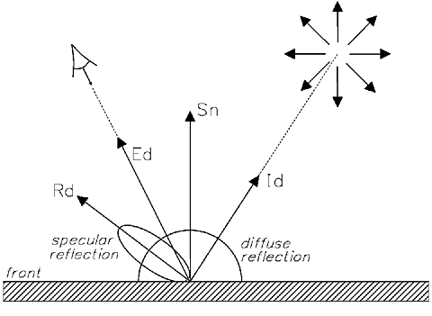
The figure, "Reflected Light Definition," illustrates the second step in the lighting calculation process.

The Reflectance Equation

The light reflected from an area geometry is the summation of the light reflected from each individual light source. For ambient light sources, the j^th component of the reflected light is equal to the summation of the following quantity over all active ambient light sources:

a_c   I_j   D_j  for  j = 1,2,3

where:

a_c is the ambient reflection coefficient of the surface

I_j is the j^th component of the incident light

D_j is the j^th component of the surface's diffuse color.

For all other light source types, the reflected light is equal to the sum of the diffuse and specular terms.

The diffuse term is defined to be the summation of the following quantity over all active light sources (other than ambient):

d_c   D_j   I_j  (S_n · I_d )  for  j = 1,2,3

where:

d_c is the diffuse reflection coefficient of the surface

D_j is the j^th diffuse color component of the surface

I_j is the intensity of the incoming ray of light

I_d is the direction of the incoming ray of light

S_n is the unit reflectance normal of the illuminated point.

When the dot product (S_n · I_d ) is less than zero, it is treated as zero and so the light source does not contribute to this term.

The specular term is defined to be the summation of the following quantity over all active light sources (other than ambient):

s_c   S_j   I_j  (E_d · R_d )^s_e   for  j = 1,2,3

where:

s_c is the specular reflection coefficient of the surface

s_e is the specular reflection exponent of the surface

S_j is the j^th specular color component of the surface

I_j is the j^th intensity component of the incoming ray of light

E_d is the unit direction vector from the illuminated point to the observer

R_d is the unit direction vector of the reflected ray of light calculated as follows:

R_d = 2 (S_n · I_d ) S_n - I_d

When either the dot product (E_d · R_d ) or the dot product (S_n · I_d ) is less than zero, it is treated as zero and so the light source does not contribute to this term.

Face-dependent Lighting Effects

The face-dependent lighting method is based on the real-world effect that causes shadows. If a light is on one side of an opaque object and the viewer is on the other side, then the viewer would not see any illumination from the light. The viewer's side would be dark, or in the shadows, or at least not as bright as the side facing the light.

The lighting process creates this effect by first determining where the lights and viewer are, then changing some of the values in the lighting calculation if viewer and lights are on opposite sides.

Use the Set Face Lighting Method (GPFLM) attribute subroutine to enable this effect through 2=FACE_DEPENDENT. (By default, the effect is off; i.e., lighting is 1=FACE_INDEPENDENT since the relationship of lights and viewer to the area is ignored).

When the Face Lighting Method is 2=FACE_DEPENDENT , then:

• Position Relationships

  The relationships of the positions of the viewer and the lights to the area is determined by calculations of various vector cross-products; the results define the orientation of the position to the face.

  • Viewer Position

    The position of the viewer is used with the geometric normal to determine the viewer orientation to the front face of the area. An object is front-facing if the geometric normal is pointing to the viewer.

  • Light Position

    The Light Source Representation table defines a position for each light that enters into the lighting calculations. You use this light position with the geometric normal to determine the orientation of the light to the front face of the area. The light is then determined to be on the front or back side.

    Note: The use of the geometric normal to determine the orientation of the light relative to the front face of the area may have a performance impact. For this reason, an approximation may be performed using the vertex normal rather than the geometric normal. The two normals are close in value for most situations, so this approximation yields good results without degrading performance.

• Lighting Calculations

  From the above processing, the position relationships of the viewer and light to the area are determined. If the light and the viewer are on opposite sides of the area, then the diffuse and specular terms of the lighting processing are suppressed (i.e. the values are set to 0). Only these two terms of the lighting calculations are affected since they are the only terms whose reflection is dependent on the position of the light source.

The effects of face-dependent lighting can be summarized based on the relationships of the light and the viewer to the front and back faces of the area.

• Light and viewer both on front side

  All lighting calculations proceed as defined.

• Light on front side, viewer on back side

  Diffuse and specular terms are both set to 0. All other lighting calculations proceed as defined.

• Light on back side, viewer on front side

  Diffuse and specular terms are both set to 0. All other lighting calculations proceed as defined.

• Light and viewer both on back side

  Back-side vertex normals are calculated by inverting the vertex normals. These back-side vertex normals are then used in the lighting calculations.

Performance Impact of Implicit Normals

The geometric normal can be explicitly provided in some primitives, or can be implicitly generated by calculations performed by the graPHIGS API Because implicit normals must be generated on every traversal, a performance impact may result. Therefore, your application programs should provide explicit normals for lighting and Hidden Line/Hidden Surface Removal (HLHSR) processing. 

Shading

The Set Interior Shading Method (GPISM and GPBISM) subroutines define how to fill the interior of area primitives. Except for 1=SHADING_NONE , the shading methods use interpolation to perform the fill process. Interpolation is the process of calculating data at intermediate points along at primitive's geometry from data at the primitive's vertices. It results in averaging the data across a primitive, typically from data defined at each vertex.

The Interior Shading Method options are:

1=SHADING_NONE

This method is the default. It specifies that no shading is to be done.

This shading method is traditionally known as "flat" shading because the same color is used everywhere on the facet.

A single color value is used everywhere for the interior color of the primitive. The method for determining the color used is described in "Color Selection". If lighting calculations are enabled, then a lighting calculation is performed on the color value.

2=SHADING_COLOR

This method specifies that shading is done by the interpolation of color values across the interior of the primitive.

This shading method is traditionally known as "Gouraud" shading, and appears as colors that blend from one vertex to another.

If lighting calculations are enabled, then a lighting calculation is performed on the color value at each vertex. The method for determining the colors used is described in "Color Selection". The resulting colors are linearly interpolated across the primitive.

If 2=SHADING_COLOR is used but no vertex color values are specified, the Interior Shading Method defaults to 1=SHADING_NONE

3=SHADING_DATA

This method specifies that shading is done by the interpolation of the data mapping data values before they are converted into colors.

If lighting is enabled, then a lighting calculation is performed on each vertex, independent of the data and colors. The data values are then linearly interpolated across the primitive along with these independent lighting calculations. Next, the interpolated data values are used to determine the color values of the interior of the primitive. Finally, these interior colors are combined with the interpolated lighting calculations to produce a lit, texture mapped interior.

If 3=SHADING_DATA is used with the data (texture) mapping method (1=DM_METHOD_COLOR ) and no vertex colors are specified, the method defaults to 1=SHADING_NONE

When Color Values Are Used As Data Values
There are instances when data values may not be used during Color Selection. Specifically, the highlighting color or pattern may be used, or the data mapping index may select 1=DM_METHOD_COLOR (See "Color Selection"). In such instances, the colors themselves are used as data mapping data values. Processing occurs as follows:

If lighting is enabled, then:

• the lighting calculations are performed independently from the colors
• the colors and lighting calculations are interpolated independently
• the interpolated values are combined at the very end to determine the interior color values
• the resulting appearance is very similar to that of 2=SHADING_COLOR

Set Lighting Calculation Mode

The Set Reflectance Model (GPRMO) and Set Interior Shading Method (GPISM and GPBISM) subroutines give you more flexibility over the graPHIGS API lighting and shading controls. However, for compatibility, the Set Lighting Calculation Mode (GPLMO) is also available.

Conceptually, the lighting calculations described here are performed for every point on an area geometry.     However, to utilize workstation capabilities and obtain the required performance, your application can control the lighting process through the Set Lighting Calculation Mode (GPLMO) subroutine which creates a structure element with one of the following values:

1=NONE

No lighting calculation is performed in this mode. Colors determined by the color selection stage are passed to the depth cueing stage with no modification. This mode is the traversal default of the graPHIGS API

Note: This mode does not necessarily mean that area geometries are displayed with a constant color. Depending on your workstation, interpolation of vertex colors and depth cueing may still be applied to the primitive.

2=PER_AREA (at least one for an area geometry)

At least one lighting calculation is performed for each area. The resultant color is assigned to all points of the area. The point where the lighting is performed is workstation dependent. Possible alternatives are:

• the first vertex
• the center of gravity
• an arbitrary vertex.

This mode does not necessarily mean the area geometry is displayed with a constant color and does not inhibit performing more lighting calculations. For polygons with vertex colors, lighting calculations may be performed for every vertex even in this mode.

3=PER_VERTEX (at least for every vertex)

Lighting calculations should be performed at least for all vertices of the area geometry. Colors of other points will be obtained by interpolating resultant colors at vertices.

Hidden Line/Hidden Surface Removal (HLHSR)

Hidden Line / Hidden Surface Removal (HLHSR) is a process used to enhance the display of 3-dimensional objects: by controlling how objects that are closer to the viewer are rendered with objects that are farther from the viewer, the application can achieve certain desired effects. For example, the application can cause hidden parts to not appear on the display, or it can display the hidden parts in a special way that indicates to the user that the parts are hidden.

HLHSR is typically implemented using a Z-buffer. A Z-buffer is storage that holds the Z-value of a pixel: this value is used to compare with other pixel Z-values that are generated during the rendering process. The comparison determines whether the frame buffer and/or the Z-buffer are to be updated with the new pixel or are to remain unchanged.

For example, consider a common HLHSR process of removing hidden surfaces. As each pixel of a surface primitive is generated, its Z-coordinate value is compared to the Z-coordinate value in the Z-buffer (if a Z-value already exists). If the new Z-value is closer to the viewer, then the new pixel value replaces the current pixel value in the frame buffer and the Z-buffer is updated with the Z-value of the new pixel. If the new Z-value is farther from the viewer, then the new pixel value does not replace the current pixel value. The effect is that closer objects overwrite objects that are farther away, hiding them. Note that both the frame buffer and the Z-buffer are updated if the comparison indicates that the new pixel should replace the existing pixel.

The Set HLHSR Identifier element is used to specify how each geometric entity is to be processed in the HLHSR process. The following table lists the HLHSR identifiers and summarizes the effect of the frame buffer and Z-buffer.

Table 8. HLHSR Processing

Identifiers 1-5 define special HLHSR effects:

1=VISUALIZE_IF_NOT_HIDDEN

If the Z-value of the generated pixel is closer to the viewer or the same distance as the Z-buffer value, then both the Z-buffer and the frame buffer are updated with the generated pixel value. This causes closer objects to overwrite farther objects.

2=VISUALIZE_IF_HIDDEN

If the Z-value of the generated pixel is farther from the viewer than the Z-buffer value, then only the frame buffer is updated with the generated pixel value, and the Z-buffer is not updated. This causes hidden objects to be displayed, but they do not update the Z-buffer since they are not closer to the viewer.

3=VISUALIZE_ALWAYS

The frame buffer is updated with the generated pixel value. In addition, if the Z-value of the generated pixel is closer to the viewer or the same distance as the Z-buffer value, then the Z-buffer is updated with the generated Z-value. This causes all objects to be displayed, but they do not update the Z-buffer unless they are closer to the viewer.

4=NOT_VISUALIZE

If the Z-value of the pixel is closer to the viewer or the same distance as the generated Z-buffer value, then the Z-buffer is updated with the generated pixel Z-value. The frame buffer is not updated. This causes no objects to be written to the frame buffer, and objects do not update the Z-buffer unless they are closer to the viewer.

5=FACE_DEPENDENT_VISUALIZATION

For back-facing areas, the frame buffer and Z-buffer are updated if Z_prim > Z_buf .

For all other entities (front-facing areas and non-area defining entities), the frame buffer and Z-buffer are updated if Z_prim >= Z_buf .

This definition is useful for the processing of coincident geometries. Consider the silhouette edges of solid objects, where the front-facing geometry meets the back-facing geometry, and assume that a front-facing area is already rendered in the frame buffer and Z-buffer and a back-facing area is then processed. Where the two areas have equal Z-values (for example, at the shared edge), then the front-facing pixels are not replaced by the back-facing pixels, (even though the back-facing area is at equal Z-value and rendered later). Otherwise, back-facing colors would "pop" out onto the front-facing area at the shared edge. The effect of this definition is to give preference to front-facing primitives over back-facing primitives when the Z-values are equal.

The front face of an area is defined by the geometric normal. If the geometric normal is pointing to the viewer, then the object is front-facing. The geometric normal can be explicitly provided in some primitives, or can be implicitly generated by calculations. Since implicit normals must be generated on every traversal, a performance impact may result. Therefore, your application programs should provide explicit normals for lighting and HLHSR processing.

The overall effect of HLHSR processing is that, except for VISUALIZE_IF_HIDDEN processing, closer objects are in the Z-buffer, and the HLHSR processing controls whether these are the objects in the frame buffer (i.e. whether these objects are displayed.)

Generation of the Z-value of a pixel is a process that depends on the primitive rendered, its transformation state, and the hardware that is used by the workstation. Conceptually, each unique pixel represents a single value out of a range of potential Z-values that the primitive can generate. This value is dependent on the method of generation that the hardware uses. For example, line primitives may generate different Z-values than a polygon primitive at the same pixel, even though the primitives use the same coordinates and transformations (and thus the pixel is conceptually the same). In large part, these differences are due to the way that the workstation hardware implements the transformation facilities and how the calculated floating-point values are converted to integer values that the hardware may use. Due to these differences, inaccuracies are possible that may give unpredictable results in some situations.

HLHSR processing of surfaces has an additional consideration. In general, a surface is tesselated into polygons for processing. This tessellation is an approximation of the conceptual surface, and the resulting polygons will not correspond at each pixel as the theoretical surface would. Thus, it is unpredictable how two close surfaces will display during HLHSR processing as a result of tesselation.

Since the hardware that implements HLHSR may be different on different workstations, see The graPHIGS Programming Interface: Technical Reference for any restrictions on HLHSR processing.

In the graPHIGS API products, the term "hidden or not hidden" is defined in the NPC of each view. A geometric entity in one view does not affect the HLHSR process of other views. Whether a given geometric entity is hidden or not is determined by whether there is any other geometric entity that has the same Normalized Projection Coordinates (NPC) X and Y values, but larger NPC Z coordinates. If there is such an entity, then the given entity is hidden. Otherwise it is not hidden.

Whether the HLHSR process should be performed or not and/or how the HLHSR checking should be performed is controlled by the HLHSR Mode of a view. The HLHSR Mode is controlled using the Set Extended View Representation (GPXVR) subroutine, which takes one of the following values:

1=OFF

In this mode, no HLHSR processing is performed. The HLHSR identifier attribute is ignored and all geometric entities are always visualized.

2=ON_THE_FLY

In this mode, the HLHSR checking is performed on the fly, i.e. when a geometric entity is processed. Whether part of the geometry is hidden or not is determined by geometric entities that have already been processed within the view. This mode corresponds to the Z-buffer technique.

HLHSR of Glyphs, Lines and Edges

Conceptually, HLHSR for these geometric entities should be performed by treating them in their mathematical sense. For example, whether an annotation text primitive is hidden should be determined only by whether the annotated reference point is hidden. When the point is hidden, the entire annotation text will be considered as hidden. However, the effects of HLHSR on these geometric entities is workstation-dependent.

Annotation Text and Marker HLHSR Procopt

If you desire not to have annotation text or markers hidden even if the reference point is hidden, use the HLHSR coordinate system processing option (PNTHLHSR). This procopt gives you the option of specifying HLHSR processing in Device Coordinates (DC) or Viewing Coordinates (VC) for annotation text and markers. Specify 2=DEVICE_COORDINATES in PNTHLHSR when you want  annotation text or marker primitives processed on a per-pixel basis in DC with the effect that text and marker strokes are z-buffered, not their reference point. Specify 1=VIEWING_COORDINATES when you want HLHSR processing of annotation text or marker primitives based on their reference point only. For a general description of the format of this procopt, see The graPHIGS Programming Interface: Technical Reference

HLHSR of Coincident Geometries

Several objects can occupy (or be intended to occupy) the same coordinate space during HLHSR processing. The resulting display depends on the types of primitives, the transformation of the primitives, and on the HLHSR implementation in the workstation.

Although two different objects may conceptually occupy the same coordinates (in the mathematical sense), the effects of floating-point inaccuracies may make the display unpredicatable in some cases. A Z-buffer in a workstation may be implemented in hardware using integer values. The floating-point Z-coordinate values must be converted to this integer format. Two floating-point coordinates that differ slightly in value may be represented by the same integer in the Z-buffer. These primitives are coincident during the HLSHR processing, and certain situations may cause unintended results to appear on the display. Likewise, two primitives that are intended to be coincident may not be when the transformed floating-point coordinates are used for HLHSR processing as they may be represented by slightly different integer values in the Z-buffer. In addition to the floating-point-to-integer conversions, different primitives may generate differing Z-values for the same pixel due to the method of generation of the pixel values from the input coordinates. For example, area-fill methods may generate different values compared to line-generation methods for the same pixel.

When the transformation processing produces Z-buffer values that are equal (based on the resolution of the value used for the Z-buffer comparison), the resulting pixels are coincident. FACE_DEPENDENT_ VISUALIZATION is provided to enhance the processing of coincident primitives. The effect of this processing during the rendering of a coincident pixel is:

    If the primitive is not a polygon whose geometric normal faces
    away from the viewer, then the pixels are written to the Z-buffer.
    If the pixels are coincident with the Z-buffer values
    (i.e. a primitive later in the traversal process overwrites
    any existing primitive that is at the same Z-location.)
    However, if the primitive is a polygon whose geometric normal
    faces away from the viewer, then the coincident pixels are
    not written to the Z-buffer.

The following examples illustrate the effects of processing primitives that have coincident geometries when using 5=FACE_DEPENDENT_VISUALIZATION processing:

• Two objects are the same: Where two objects are the same, the objects have exactly the same definition data, are in exactly the same transformation environment, and generate the same geometric entities. For example, an application could execute a structure that contains a solid-filled polygon, change the interior color, then execute the polygon structure again. The effect of the above processing is that, except for polygons with a normal that face away from the viewer, the primitive processed last always overwrites existing coincident primitives. However, a polygon with a normal that faces away from the viewer will not overwrite other coincident primitives already in the Z-buffer.
• Two objects intersect: Where two objects intersect, they share some of the same pixels with the same Z-value. For example, 2 distinct polygons can be defined that share a common edge. This common edge is rendered according to the same processing described above as each of the 2 polygons are processed. However, note that inaccuracies in floating-point calculations may cause 2 objects that "should" intersect (in the theoretical sense) to actually have slightly differing Z-values, thus changing their relationship during Z-buffer processing. To work consistently, the two intersecting primitives must have exactly the same definition data at the intersection, be in exactly the same transformation environment, and generate the same geometric entities for all types of HLHSR processing.

• One object completely contains another object: One object completely containing another occurs, for example, when a smaller polygon is drawn on a larger polygon, or when a line is drawn over the interior of a polygon. In general, floating-point inaccuracies make the HLHSR processing of included objects unpredictable. The rendering to the Z-buffer on a pixel-by-pixel basis may result in pixels from either primitive being displayed. HLHSR processing cannot guarantee that the later primitive overwrites any former primitive since the value of any pixel's Z-coordinate may be affected by the floating-point inaccuracies.
• A line drawn on the edge of a polygon: In general, floating-point inaccuracies make the HLHSR processing of a line drawn on the edge of a polygon unpredictable. To guarantee that a line is drawn on the polygon edge, the application can use the Edge Flag attribute of 2=ON is 2=ON , the edge produces the desired line around the polygon, and the edge line is rendered properly with respect to the pixels of the interior, boundary, and background.

  lf the application cannot use edges and must draw a polyline around the polygon, then the application can use the Edge Flag of 3=GEOMETRY_ONLY This will generate the polygon in the frame buffer in the same manner as with Edge Flag 1=OFF , but will generate the polygon in the Z-buffer using both a line-generation method and an area-fill method, which ensures that the Z-buffer contents will be consistent with the following polylines. (The Z-buffer is not guaranteed to be consistent with the following polylines if the Edge Flag is 1=OFF since the Z-buffer contents are generated by an area-fill algorithm. These Z-buffer values may differ unpredictably along any coincident pixels that the polyline will generate; thus pixels from the interior may randomly "bleed-through" the polyline. The 1=GEOMETRY_ONLY processing will guarantee that the Z-buffer contents of the boundary of the polygon are consistent with the Z-buffer contents that a line-generation method generates for the same points). To work consistently, the following polyline must have exactly the same definition data and be in exactly the same transformation environment; the following polyline will then be coincident with the boundary of the polygon, and the polyline pixels will replace the polygon pixels.

Z-Buffer Controls

Some workstations are able to inhibit the updating of the Z-buffer. This capability may be useful when doing special HLHSR (hidden line, hidden surface removal) processing using the Z-buffer. The Set Z-buffer Protect mask (GPZBM) attribute provides application control of updates to the Z-buffer by use of a Z-buffer mask. When the mask value is zero for all 32 bits, then the Z-buffer is updated normally. When the mask value is one for all 32 bits, then the Z-buffer is not updated.

Currently, the only defined values for the mask bits are

• all bits are zero, or
• all bits are one

Any non-zero mask value is treated as if a mask of one for all 32 bits had been specified. However, applications should not use values other than the defined values to allow for possible future definition of additional values.

The Z-buffer protect mask controls the Z-buffer update independent of the HLHSR identifier. If the specified HLHSR identifier defines that the Z-buffer is to be udpated and the Z-buffer protect mask prohibits updates to the Z-buffer, then the Z-buffer is not updated.

The Z-buffer Protect Mask (GPZBM) structure element is defined as a Generalized Structure Element (GSE) and may not be supported on all workstations.

Examples

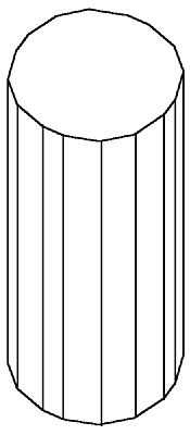
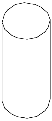
A cylinder can be approximated by a set of polygons defined by the following three structures:

1. A structure containing all polygon definitions.
2. A structure containing all edges of the top and bottom discs which are represented by polylines.
3. A structure containing all edges on the cylindrical surface which are represented by polyhedron edge primitives with appropriate normal vectors, i.e. normal vectors of adjacent polygons.

The following pages contain pseudo code examples illustrating the use of HLHSR and polyhedron edge culling.

  Set edge flag (on)
  Set HLHSR identifier (not visualize)
  Execute structure (polygons)
  Set HLHSR identifier (visualize when not hidden)
  Set line style (solid)
  Execute structure (edges of discs)
  Execute structure (edges of cylinder)

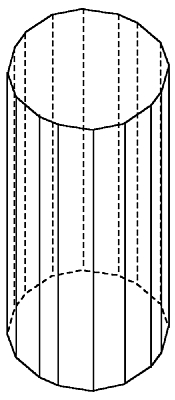
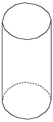
  Set edge flag (on)
  Set HLHSR identifier (not visualize)
  Execute structure (polygons)
  Set HLHSR identifier (visualize when hidden)
  Set line style (dotted)
  Set polyhedron edge cull mode
  Execute structure (edges of discs)
  Execute structure (edges of cylinder)
  Set HLHSR identifier (visualize when not hidden)
  Set line style (solid)
  Execute structure (edges of discs)
  Execute structure (edges of cylinder)

If you want to eliminate the edges on the cylindrical surface except those which form the outline, your application can combine polyhedron edge culling with HLHSR.

  Set edge flag (on)
  Set HLHSR identifier (not visualize)
  Execute structure (polygons)
  Set HLHSR identifier (visualize when not hidden)
  Set line style (solid)
  Set polyhedron edge culling mode (both back or both front)
  Execute structure (edges of discs)
  Execute structure (edges of cylinder)

  Set edge flag (on)
  Set HLHSR identifier (not visualize)
  Execute structure (polygons)
  Set HLHSR identifier (visualize when hidden)
  Set line style (dotted)
  Execute structure (edges of discs)
  Set HLHSR identifier (visualize when not hidden)
  Set polyhedron edge culling mode (both back or both front)
  Set line style (solid)
  Execute structure (edges of discs)
  Execute structure (edges of cylinder)

Depth Cueing

Depth cueing is the process of adjusting the color of locations on a primitive based on the NPC Z coordinate of that location. For example, a primitive could fade in color into the distance so as to give the illusion of depth. Depth cueing applies to all primitives.

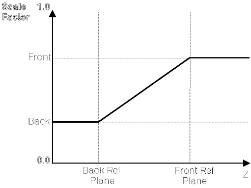
The Depth Cue Mode can be set to either 1=SUPPRESSED or 2=ALLOWED , which enables or disables the effect of depth cueing. Note that depth cueing can be activated even when no hidden line/hidden surface removal (HLHSR) is performed or when shading and lighting are turned off. Depth cueing is independent of all other controls. The depth cue reference planes field consists of two Z values in NPC space which define two planes parallel to the XY plane in NPC. These are referred to as the front and back reference planes. The depth cue scale factors are two values from 0.0 to 1.0 that determine the amount of the input color and depth cue color that are to be mixed. The scale factor varies linearly between the front and back reference planes. The figure, "Depth Cue Scale Factor," illustrates how the depth cue scale factor varies with Z in NPC.

The Z coordinate of the location at which depth cueing is being calculated is used to compute the scale factor to be used in the following equation. If the z position is not between the front or back reference planes, the scale factor of the closest reference plane is used. The scale factor is used as a ratio of the input color to the depth cue color. Mathematically, this is:

c = s_f c_i + (l - s_f) c_d

where:

c is the color component (Red, Green, or Blue) of the resulting color

s_f is the depth cue scale factor

c_i is the color component entering the depth cue stage of the rendering pipeline

c_d is the color component of the depth cue color.

The entries of the depth cue table are set by the Set Depth Cue Representation (GPDCR) subroutine. Entry 0 of the depth cue table contains a depth cue mode of suppressed and cannot be modified. If only one entry exists, depth cueing is therefore not supported. The number of depth cue table entries for a workstation can be determined with the Inquire Depth Cue Facilities (GPQDCF) subroutine.

Transparency

The interior of an area geometry with non-zero transparency coefficient is called a transparent surface processing of the transparent surface is controlled by a view's transparent processing mode set by the Set Extended View Representation (GPXVR) subroutine. This mode takes one of the following four values:

1=OFF (default)

The transparency coefficient is ignored.

2=PARTIAL_TRANSPARENT

Use this to create "screen-door" transparency. A transparent surface is treated as a surface with many small holes. The number of holes generated and the arrangement of the holes are workstation-dependent, therefore they may vary according to the transparency coefficient or may be fixed independent of the coefficient. As the transparency coefficient approaches 1.0, fewer pixels are generally written to the frame buffer. The generated primitive is totally transparent when none of its pixels is written to the frame buffer.

Use GPQTMO to inquire this and other Transparency Mode facilities for your workstation.

3=BLEND

Use this to combine the colors of the area primitive being rendered (the source colors) with previously rendered output (the destination colors) to create a new color.

Note: Use 3=BLEND for area primitives such as polygons. If you want to blend all primitives, use 4=BLEND_ALL

Alpha Blending: The destination blending coefficient, also called the alpha value (a_dest) and used in the blending operation, is an integer in the range of 0 to 255 expressed as:

a_dest = 255 × (1.0 - coeff)

The transparency coefficient (coeff) is a floating point value in the range of 0.0 to 1.0. You can assign an amount of transparency to objects by specifying the value of the coeff parameter using the Set Transparency Coefficient (GPTCO), the Set Back Transparency Coefficient (GPBTCO) or the Set Surface Properties (GPSPR) subroutines.

The source blending coefficient or alpha value (a_src ) used in the blending operation is calculated from the source transparency coefficient (0.0 to 1.0) and expressed as:

a_src = 1.0 - coeff.

The terms COLOR_src and COLOR_dest are used to refer to the respective terms of R_src, G_src, B_src, and a_src , and of R_dest, G_dest, B_dest, and a_dest .

Specifically:

COLOR = (srcf × COLOR_src) + (destf × COLOR_dest)

is equivalent to:

R = (srcf × R_src) + (destf × R_dest)

G = (srcf × G_src) + (destf × G_dest)

B = (srcf × B_src) + (destf × B_dest)

a = (srcf × a_src ) + (destf × a_dest )

The source and destination blending functions specify the methods used to blend the source and destination colors. These are specified using the Set Blending Function (GPBLF) and Set Back Blending Function (GPBBLF) subroutines.

Table 9 defines the source and destination functions supported by the GPBLF subroutine the number and availability of source and destination blending functions on your workstation.

Table 9. Blending Functions

Source and destination blending functions.
Source function id	srcf	Destination function id	destf
1	0	1	0
2	1	2	1
3	asrc	3	asrc
4	1 - asrc	4	1 - asrc
5	adest	5	adest
6	1 - adest	6	1 - adest
7	Rdest , Gdest , Bdest , or adest	7	Rsrc , Gsrc , Bsrc , or asrc
8	1 - (Rdest, Gdest, Bdest, or adest)	8	1 - (Rsrc, Gsrc, Bsrc, or asrc)
9	min (asrc, 1 - adest)

For example, if srcf has the default value 3=SRCBF_SRC_ALPHA and destf has the default value 4=DSTBF_ONE_MINUS_SRC_ALPHA , then the blending function becomes:

COLOR = (a_src × COLOR_src) + ((1 - a_src) × COLOR_dest)

During blend processing, the color attributes bound to the primitive define the color values. These colors, therefore, can be indexed (indirect) or direct, or the result of color modifications (e.g., lighting and/or shading) applied in the rendering pipeline.

4=BLEND_ALL

Use this value to blend all primitives.

Note: Use 3=BLEND for area primitives such as polygons. If you want to blend all primitives, use 4=BLEND_ALL

Blending Antialiased Lines: For BLEND_ALL , the values used for each of the two pixels generated for each point along the antialiased line is calculated as the proportional coverage of each antialiased pixel using the line's end-points and slope. The interpolated alpha a is attenuated by this proportional coverage. If the interpolated alpha value is denoted by a_int and the pixel's proportional coverage is denoted by c, then the resulting alpha (a_src), is described by the expression:

a_src = a_int × c

The result (a_src) is used in the following classical antialiasing blend operation:

COLOR = (a_scr × COLOR_scr) + (( 1 - a_src) × COLOR_dest)

a = a_src

Specifying Initial Shield Alpha Value

Use the Set Extended View Representation (GPXVR)  subroutine to specify an initial alpha value for a view's shield. For more information on the shield alpha value and the GPXVR subroutine, see Chapter 15. "Advanced Viewing Capabilities".

Specifying Alpha Values for Primitives

For 3=BLEND and 4=BLEND_ALL you specify the transparency coefficient as a parameter with the following area primitives:

• Polygon 2 With Data (GPPGD2)
• Polygon 3 With Data (GPPGD3)
• Triangle Strip 3 (GPTS3)
• Quadrilateral Mesh 3 (GPQM3)
• Polyline Set 3 With Data (GPPLD3)

The remainder of the rendering pipeline deals with the processing of colors which is discussed in detail in the next chapter.

Texture/Data Mapping

Overview of Texture/Data Mapping

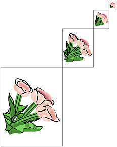
Texture mapping is a method of filling the interior of area primitives from a collection of colors.  An example of texture mapping is a digitized photograph image which is mapped onto a polygon. You use the data mapping facilities of the graPHIGS API to perform texture mapping.

Texture mapping and data mapping perform the same fundamental operations, as shown in the figure, "Texture Mapping / Data Mapping Operations." In texture mapping, data specified on the vertices of primitives define the location and orientation of a texture image vertex data values, known as texture coordinates, are first modified by a texture coordinate matrix and transformed into a predefined texture coordinate scale, traditionally in the range of 0.0 to 1.0. The texture coordinates are then used to index into the texture image to determine the color at each pixel of the displayed primitive.

In data mapping, application data values such as temperature, stress, seismic readings, or particle density are measured at each primitive vertex. These vertex values are known simply as data mapping data scaled according to specified data range limits mapping values are then used to index a color list (or set of color lists) in the data mapping representation table, to determine each pixel color as the primitive is displayed.

The primitives that support vertex data mapping data are:

• Polygon 2 With Data (GPPGD2)
• Polygon 3 With Data (GPPGD3)
• Triangle Strip 3 (GPTS3)
• Quadrilateral Mesh 3 (GPQM3)

Interior Shading Method

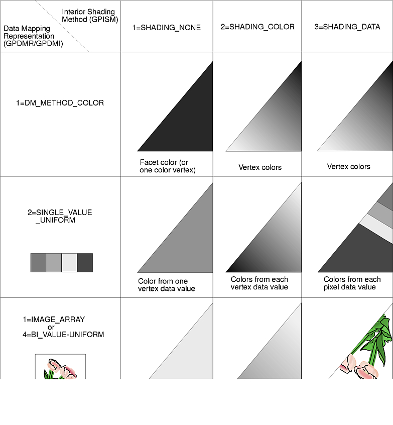
Depending on the option you specify in the Set Interior Shading Method (GPISM and GPBISM) subroutines for an area primitive (see "Shading"), the graPHIGS API uses vertex data to determine the color of each facet (1=SHADING_NONE ) or each vertex (2=SHADING_COLOR ). The third shading method (3=SHADING_DATA ) interpolates vertex data, producing data values that determine the color at every pixel of the rendered primitive. Method 3=SHADING_DATA is used for texture mapping. "Lighting, Shading, and Color Selection" describes how data mapping and shading work in the graPHIGS API rendering pipeline.

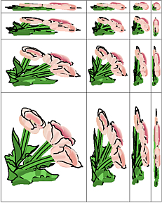
The figure, "Data (Texture) Mapped Primitive Examples," shows data (texture) mapped primitives using the three shading methods (GPISM) in conjunction with each of the data mapping methods (GPDMR)

Data Mapping Method

The data mapping methods supported through the Set Data Mapping Representation (GPDMR) subroutine:

1=DM_METHOD_COLOR

specifies that the color is determined directly from the color values of the primitive; data mapping is not performed.

-1=IMAGE_ARRAY

uses a pair of data values to select a color from an array of colors. This data mapping method supports mipmapping, an image filtering technique that enhances the visual quality of the texture mapped surface.

2=SINGLE_VALUE_UNIFORM

uses a single data value to select a color from a list of colors.

4=BI_VALUE_UNIFORM

uses a pair of data values to select a color from a set of color lists.

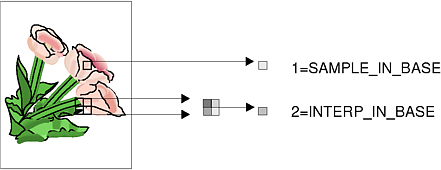
If the data mapping method selected and the contents of the  primitive are inconsistent, then the primitive is rendered using the data mapping method 1=DM_METHOD_COLOR.

Mipmapping

A mipmap image generally incorporates several color values from its "parent" image in an attempt to depict the same image at a lower resolution. For example, a red and white texture image may have pink hues in its mipmap images. This also matches human perception. That is, if a red-and-white tablecloth is on a distant table, the color appears pink from the viewer's perspective as a result of the visual blend of red and white.

Color Data Formats

The graPHIGS API uses color lists that are organized into one of five different formats. Three of these formats use simple color lists, sometimes called the base texture image formats include mipmap images derived from the base texture image.

Mipmap images can be specified for any -1=IMAGE_ARRAY base texture image whose size is defined by powers of two. Each mipmap image is half the size (in each dimension) of its parent image. The supported IMAGE_ARRAY texture image formats are BASE_DATA , SQUARE_MM , and RECT_MM

Note: Since Mipmapping does not exist in the ISO PHIGS PLUS standard methods, only base SINGLE_VALUE_UNIFORM and BI_VALUE_UNIFORM color images exist.

Texture images do not have to be square. Square mipmaps (SQUARE_MM ) are called "square" because the aspect ratio of the base texture image is maintained for all mipmap images. That is, the ratio of width to height is equal in all images. Rectangular mipmaps (RECT_MM ) are called "rectangular" because this ratio varies across mipmap images.

• -1=IMAGE_ARRAY representation method with format 1=BASE_DATA is the base or parent texture image (no mipmaps), as shown in this figure.
• -1=IMAGE_ARRAY representation method with format 2=SQUARE_MM are square filtered mipmap images, as shown in this figure.
• -1=IMAGE_ARRAY representation method with format 3=RECT_MM are rectangular filtered mipmap images, as shown in this figure.
• 2=SINGLE_VALUE_UNIFORM method color list (no mipmaps available), as shown in this figure.
• 4=BI_VALUE_UNIFORM method color lists (no mipmaps available), as shown in this figure.

Data Filtering

Bounding Method

When the data values exceed the range you specify in the data mapping representation table, you can also specify a Bounding Method that fills the "out-of-range" area within the primitive in one of two ways:

1=CLAMP

uses last color in the range for every pixel whose data value exceeds the data mapping range, or the first color in the range for every pixel whose data value is less than the data mapping range. The effect is a continuous color in the "out-of-range" fill area for both the u and v boundaries.

2=REPEAT

repeats the texture image across the area. This method is useful in representing cyclic or repetitious data.

Minification and Magnification

Data filtering methods specify which of the supplied mipmap images are to be used and how each pixel color value is determined from these images. You can specify two kinds of data filtering methods in the graPHIGS API, the minification filter and the magnification filter, using the Set Data Filtering Method (GPDFM and GPBDFM) subroutines. The minification filter maps large texture images onto small screen areas. The magnification filter maps small texture images onto large screen areas.

Depending on the filtering methods you specify, the graPHIGS API samples and/or interpolates color values from the base texture image and its mipmaps if supplied. Specifically, this process selects either the base image, a single mipmap image, or multiple mipmap images. In the latter case, the color value is interpolated between the selected mipmap images. Additionally, you can specify the selection of only one color value from each mipmap image (sampling within the mipmap image), or multiple color values (interpolating values within the mipmap image).

Data Filtering Methods: Base Image

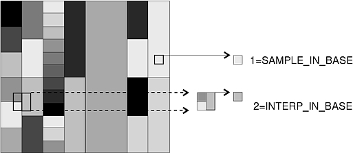
The following filtering methods specify that the graPHIGS API should use only the base texture image. These filter methods may be selected for minification or magnification and apply to any data organization format, as shown in this figure.

1=SAMPLE_IN_BASE

Selects only the base texture image. This method samples the one color value in that image which is closest to the application data values.

2=INTERP_IN_BASE

Selects only the base texture image. This method selects the four color values in that image which are closest to the application data values, then interpolates these four texture color values into a single pixel color.

Data Filtering Methods: Square Mipmaps

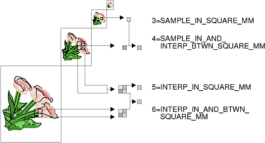
The following filtering methods specify that the graPHIGS API should use the texture image together with its square mipmaps. These filter methods may be selected for minification, and apply only to the -1=IMAGE_ARRAY data organization with 2=SQUARE_MM or 3=RECT_MM format, as shown in this figure.

Note: Rectangular mipmaps contain a complete set of square mipmaps.

3=SAMPLE_IN_SQUARE_MM

selects the single square mipmap image which most closely matches the current pixel coverage. This method samples the one color value in that image which is closest to the application data values.

4=SAMPLE_IN_AND_INTERP_BTWN_SQUARE_MM

selects the two square mipmap images which most closely match the current pixel coverage. This method samples the one color value in each image which is closest to the application data values, then interpolates these two texture color values into a single pixel color.

5=INTERP_IN_SQUARE_MM

selects the one square mipmap image which most closely matches the current pixel coverage. This method selects the four color values in that image which are closest to the application data values, then interpolates these four texture color values into a single pixel color.

6=INTERP_IN_AND_BTWN_SQUARE_MM

selects the two square mipmap images which most closely match the current pixel coverage. This method selects the four color values in each image which are closest to the application data values, then interpolates these eight texture color values into a single pixel color.

Data Filtering Methods: Rectangular Mipmaps

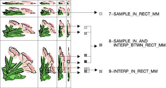
The following filtering methods specify that the graPHIGS API should use the texture image with its rectangular mipmap images These filter methods may be selected for minification only, and apply only to the -1=IMAGE_ARRAY data organization with 3=RECT_MM format, as shown in this figure.

7=SAMPLE_IN_RECT_MM

selects the one rectangular mipmap image which most closely matches the current pixel coverage. This method samples the one color value in that image which is closest to the application data values.

8=SAMPLE_IN_AND_INTERP_BTWN_RECT_MM

selects the four rectangular mipmap images which most closely match the current pixel coverage. This method samples the one color value in each image which is closest to the application data values, then interpolates these four texture color values into a single pixel color.

9=INTERP_IN_RECT_MM

selects the one rectangular mipmap image which most closely matches the current pixel coverage. This method selects the four color values in that image which are closest to the application data values, then interpolates these four texture color values into a single pixel color.

Data Filtering Methods: SINGLE_VALUE and BI_VALUE

Because SINGLE_VALUE_UNIFORM and BI_VALUE_UNIFORM color data organizations do not support mipmap images, they are similar in nature to the IMAGE_ARRAY organization with BASE_DATA format. Any data filtering methods that you can apply to IMAGE_ARRAY with the BASE_DATA format, you can also apply to SINGLE_VALUE_UNIFORM or BI_VALUE_UNIFORM color lists.

SINGLE_VALUE_UNIFORM

With a SINGLE_VALUE_UNIFORM color list, the graPHIGS API selects the color values according to the pixel's coverage in terms of the single data value u This is the same result as for an IMAGE_ARRAY representation where the vertical dimension is one since all values of v result in the same color value. This is sometimes referred to as a 1-dimensional texture image, as shown in this figure.

BI_VALUE_UNIFORM

In the case of BI_VALUE_UNIFORM , the graPHIGS API selects color values according to the pixel's coverage in both the u and v can result in the interpolation of up to four colors, depending on the number of entries in each adjacent color list. If the two adjacent color lists have only one entry apiece, then two color values are selected, as in the SINGLE_VALUE_UNIFORM example. If the color lists are of another equal length, then four color values are selected, as in the IMAGE_ARRAY examples. And if the color lists are of different lengths, then three color values may be selected; one from the shorter list, and two from the longer, as shown in this figure.

Data Filtering: Summary

Table 10 below shows the range of filtering methods supported for each of the three Data Mapping Methods in the graPHIGS API according to the color data format that is used.

Table 10. Data Filtering Summary Chart

Note:

1. If any mismatch occurs between the filtering method and the mipmap organization during traversal, the graPHIGS API uses the SAMPLE_IN_BASE filtering method instead.
2. Mipmaps must be available when methods 3 through 9 are specified.