[ Previous |
Next |
Contents |
Glossary |
Search ]
Performance Toolbox Version 1.2 and 2 for AIX: Guide and Reference
Chapter 2. Monitoring Statistics with xmperf
This chapter provides information about monitoring statistics with
the xmperf program.
You can benefit from having xmperf working while you read this
chapter. To do this, follow the instructions
in Appendix A, Installing the Performance
Toolbox for AIX to install the program and supporting files. When you
have successfully installed the files, follow these steps:
- To start the X Window System, issue the command xinit
.
- From the aixterm window, issue the command xmperf&
to start the program and make it run in the
background.
- Use the pulldown menu marked Monitor to see the list
of available monitoring devices. Click on a few to
see different ones.
- Adjust the windows opened by xmperf so that
they don't hide each other or the aixterm window.
Performance Monitoring
Monitoring the performance of computer systems is one of
the most important tasks of a system administrator.
Performance monitoring is important for many reasons,
including:
- The need to identify and possibly improve
performance-heavy applications.
- The need to identify scarce system resources and take
steps to provide more of those resources.
- The need for load predictions as input to capacity
planning for the future.
The xmperf performance monitor is a powerful and
comprehensive graphical monitoring system. It is designed to
monitor the performance on the system where it itself is
executing and at the same time allow monitoring of remote
systems via a network. Every host to be monitored by xmperf,
including the system where xmperf runs, must have the
Agent component installed and properly configured.
Note: Remote systems can only be monitored if
the Performance Toolbox Network feature is installed. If
the Performance Toolbox Local feature is installed then
only the local host can be monitored. Discussions about
remote system monitoring pertain only to the Performance
Toolbox Network feature.
In addition to monitoring performance in semi-real time, xmperf
also is designed to allow recording of performance data and
to play recorded performance data back in graphical windows.
Introducing xmperf
The xmperf program is the most comprehensive and
largest program in the Manager component of PTX. It is an X
Window System-based program developed with the OSF/Motif
Toolkit. The xmperf program allows you to define
monitoring environments to supervise the performance of the
local AIX system and remote systems. Each monitoring
environment consists of a number of consoles. Consoles show
up as graphical windows on the display. Consoles, in turn,
contain one or more instruments and each instrument can show
one or more values that are monitored.
Each xmperf environment is kept in a separate
configuration file. The configuration file defaults to the
file name xmperf.cf
in your home directory but a
different file can be specified when xmperf is
started. See Overview of
File Placement
for alternative locations of this
file.
Consoles are named entities allowing you to activate any
one or more consoles by selecting from a menu. New consoles
can be defined and existing ones can be changed
interactively. Consoles allow you to define and group
collections of monitoring instruments in whichever
configuration is convenient. Instruments are the actual
monitoring devices enclosed within consoles as rectangular
graphical subwindows.
Instruments come in two flavors:
- Recording Instruments
- The term recording does not mean that the instruments
record events to a disk file. All instrument types
have the capability to do that. It merely describes
the ability to show the statistics for a system
resource over a period of time. Recording instruments
have a time scale with the current time to the right.
The values plotted are moved to the left as new
readings are received.
-
- State Instruments
- State instruments show the latest statistics for a
system resource, optionally as a weighted average.
They do not show the statistics over time but collect
this data in case you want to change the instrument
to a recording instrument.
All instruments are defined with a primary graph style.
The following graph styles are currently available:
Recording graphs:
- Line graph
- Area graph
- Skyline graph
- Bar graph
State graphs:
- State bar
- State light
- Pie chart
- Speedometer
All instruments can monitor up to 24 different statistics
at a time. Each statistic is represented by a value. Values
can be selected from menus of available statistics. Depending
on your system and the availability of tools, statistics
could be local or remote.
To illustrate these concepts, think of a hypothetical
example (illustrated in the figure Sample
xmperf Console) of a console defined to contain
three instruments as follows:
State instrument, shaped as a pie chart, showing three
values as a percentage of total memory in the local
system:
- Free memory
- Memory used for computational segments
- Memory used for non-computational segments
Recording instrument, plotted as a state bar graph,
showing four values:
- Percent of CPU time spent in kernel mode
- Percent of CPU time spent in user mode
- Percent of CPU time spent waiting for disk
input/output
- Percent of CPU time spent in idle state
Recording instrument, plotted as a line graph,
showing:
- Number of page-ins per second
- Number of page-outs per second
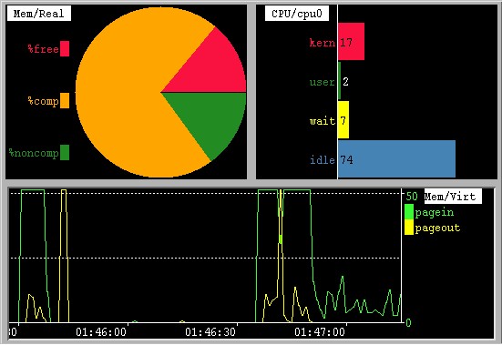
Sample xmperf Console
In addition to the monitoring features, xmperf also
provides an enhanced interface to system commands. You
configure the interface by editing the xmperf
configuration file. Commands can be grouped under either of
three main menu items:
- Analysis
- Controls
- Utilities
As another convenience to you, xmperf also can be
used to display a list of active processes in the system. The
list can be sorted after a number of criteria. Associated
with the process list is yet another user-configurable
command menu. Commands defined here take a list of process
IDs as argument.
Monitoring Hierarchy
Whenever you start xmperf, you must supply a
configuration file to define the environment in which you
want to do the monitoring. The file may be an empty
(zero-length) file, in which case you must define the
environment from scratch. If no file is specified, xmperf
defaults to the file xmperf.cf
in your home
directory. If the file does not exist in your home directory,
it is searched for as described in Overview of File Placement
.
Normally, the configuration file defines one or more
consoles, each typically used to monitor a related set of
performance data. For example, one console might be called
"Network" and provide one graph for each network
interface in the system. Another might be called
"Disks" and contain graphs to show the activity of
each physical disk and the types of input/output requests.
The configuration file, thus, defines the environment and
contains one or more definitions of consoles. Together they
constitute the top two levels in the hierarchy. The third
level is the subdivision of consoles into instruments. Using
the "Network" example from above, this console
might have an instrument defined for each of your system's
network interfaces. This way, whenever you want to check the
network load, you simply call a monitoring console by its
name, in this case "Network," and monitoring starts
immediately.
Returning to the example of network monitoring, obviously,
there's more than one thing to keep an eye on for each of the
network interfaces in a system. You might want to monitor the
number of retransmissions and probably want to know how much
network load comes from input and how much from output. Those
are just a couple of the many types of data that might
interest you. In xmperf terms, each data type is
referred to as a value and represents a flow of data
from one particular type of statistics collected by the
system. If each of these data values had to be monitored in
separate instruments, it would be difficult to correlate them
and you'd end up with an unmanageable number of instruments
for even simple monitoring tasks. Therefore, an instrument
can be made to monitor more than one value so that each
instrument monitors a set of data values. Values comprise the
fourth level in the monitoring hierarchy.
Statistics and Values
A given system, at any point in time, has a number of
system resources that do not change between boots. Such
resources include, but are not limited to, the following:
- Processing units
- Real memory
- Non-removable disk drives
- Network interfaces
Your system collects a large amount of performance-related
statistics about such resources. This data can be accessed
from application programs through the APIs provided by PTX.
One such application program is xmperf. It provides a
user interface that allows you to select the data to monitor
from lists of the data available. By selecting multiple data
values, you can build instruments where multiple statistics
can be plotted on a common time scale for easy correlation.
Data Value Properties
When you select a value to monitor, you get a set of
default properties for that data value. Each property can be
changed to reflect special needs. The properties associated
with a data value and their defaults are as follows:
- Style
- A secondary graph style, which is ignored for state
graphs. By specifying a secondary graph style
different from the primary style of an instrument,
interesting effects can be created. For example, if
the instrument's primary style is a bar graph, then
you can choose a line graph style for one or more
values to plot related values so they overlay the bar
graph.
Default = Same as primary style for
instrument.
- Color
- The color used to represent the value when plotted.
If the value is displayed as a state light, the color
is used to paint the "lights" when a data
value is lower than a descending threshold or higher
than an ascending threshold.
Default = As
specified in resource file (see The xmperf
Resource File )
or (for colors not defined in
resource file) generated from colors in the color map
and contrasting from neighbor colors.
- Tile
- A pattern (pixmap) used to "tile" the value
as it is drawn in an instrument. Tiles are ignored
for line drawing, for text, and for the state light
type instruments. When tiling is used, it is always
done by mixing the color of the value and the
background color of the instrument in one out of
eleven available patterns, numbered from 1 to 11.
Default
= foreground (tile 1 = 100% foreground color).
- Scale, low
- The lowest value plotted. This property only has a
meaning for recording graphs and for the state bar
graph.
When a low scale value is given for a
recording graph or a state bar graph, then the scale
of the graph goes from the low scale value to the
high scale value. For example, if the low scale is 50
and high scale is 100, then the lowest value you will
ever see plotted in the instrument is 51. A value of
75 would extend half-way into the plotting area.
Default = From system tables, usually zero.
- Scale, high
- The value that determines the scale of the graphs. If
values are encountered that exceed the high scale
limit, the graphs are cut off to fit the plotting
area. This property has no meaning for the state
light graph type.
Default = From system tables.
- Threshold
- This property is used only for the state light graph
type. It defines the value at which the "light
is turned on." Whether the light is on when the
value is above or below the threshold is determined
by the threshold type.
Default = zero.
- Threshold Type
- This property is used only for the state light graph
type. It must be descending or ascending. If
descending, the light is turned on when the last
value received is equal to or below the threshold. If
ascending, the light is turned on when the last value
received is equal to or above the threshold.
Default
= Ascending.
- Label
- This property can be used to specify a user-defined
text that is used to label the value in the
instrument.
Default = Null (path name of value is
used, see Path Names)
.
Path Names
Many system resources exist in multiple copies. For
example, a system may have three disks, and two of those may
be used for paging space. A system may also have multiple
network interfaces, and several other resources may be
duplicated. Generally, one set of statistics is collected for
each resource copy.
Because of this duplication of statistics, the selection
of values to plot in an instrument is done through a
multi-level selection process. Since this process is
available, it is also used to group statistics even when they
are not duplicated. The unique name used to identify a value
is composed of one-level names separated by slashes, much
like a fully qualified UNIX file name. The fully qualified
name of a value is called the path name of the value. To
identify the percentage of time a particular disk on the host
system with the hostname birte is busy, the path name
might be:
hosts/birte/Disk/hdisk02/busy
For space reasons, it is seldom possible to display all of
the path name in instruments. For example, given that the
number of characters used to display value names is 12, only
the last 12 characters of the above name would be displayed,
yielding:
hdisk02/busy
The default length of a value name is 12, but you can
specify up to 32 characters using the command line argument -w.
In addition, the -a command line argument allows you
to request adjustment of the text length to what is
necessary to display the value names. When -a is used,
the text length may be less than what is specified by -w
(or the default, whichever applies) but never longer. The X
Window System resources LegendAdjust
and LegendWidth
can be used in place of the command line arguments. See The xmperf Command Line
for a description of command line options and The xmperf Resource File
for a description of supported resources.
In many cases, an instrument or a console is used to
display statistics that have some of the value path name in
common. When this happens, xmperf automatically
removes the common part of the name from the displayed name
and shows it in an appropriate place, dependent on the type
of instruments used. This is explained in Value Name Display
and The Console Title Bar
.
User-defined Labels
No matter how much thought is put into the naming of each
level in the hierarchy of statistics, you are bound to end up
with some that are not very informative. In such cases you
might want to specify your own name for a value. You can do
so from the dialog box used to add or change a value as
described in Changing
the Properties of a Value .
Instruments
An instrument occupies a rectangular area within the
window that represents a console. Each instrument may plot up
to 24 values simultaneously. The instrument defines a set of
statistics and is fed by network packets that contain a
reading of all the values in the set, taken at the same time.
All values in an instrument must be supplied from the same
host system.
The instrument shows the incoming observations of the
values as they are received depending on the type of
statistic selected. Statistics can be of types:
- SiCounter
- Value is incremented continuously. Instruments show
the delta (change) in the value between observations,
divided by the elapsed time, representing a rate per
second.
-
- SiQuantity
- Value represents a level, such as memory used or
available disk space. The actual observation value is
shown by instruments.
Instruments defined in xmperf correspond to
statsets in the xmservd daemons of the systems the
instruments are monitoring. The section on
Statsets
gives
information about statsets and their relationship to
instruments.
Configuring Instruments
Instruments can be configured through a menu-based
interface as described in The Modify Instrument
Submenu .
In addition to selecting from 1 to 24
values to be monitored by the instrument, the following
properties are established for the instrument as a whole:
- Style
- The primary graph style of the instrument. If the
graph is a recording graph, not all values plotted by
the graph need to use this graph style. In the case
of state graphs, all values are forced to use the
primary style of the instrument.
Default = Line
graph.
- Foreground
- The foreground color of the instrument. Most
noticeably used to display time stamps and lines to
define the graph limits.
Default = White.
- Background
- The background color of the instrument.
Default =
Black.
- Tile
- A pattern (pixmap) used to "tile" the
background of the instrument. Tiles are ignored for
state light type instruments. When tiling is used, it
is always done by mixing the foreground color and the
background color of the instrument in one out of
eleven available patterns.
Default = Tile 2 (100%
background color, that is, no tiling).
- Interval
- The time interval between observations. Minimum is
0.2 second, maximum is 30 minutes. Even though the
sampling interval can be requested as any value in
the above range, it may be changed by the xmservd
daemon on the remote system that supplies the
statistics. For example, if you request a sampling
interval of 0.2 second but the remote host's daemon
is configured to send data no faster than every 500
milliseconds, then the remote host determines the
speed. As explained in Rounding of
Sampling Interval
, xmservd rounds
sampling intervals so that the example above would
result in an effective sampling interval of 500
milliseconds.
Default = 5 seconds.
- History
- The number of observations to be maintained by the
instrument. For example, if the interval between
observations is 5 seconds and you have specified that
the history is 1,000 readings, then the time period
covered by the graph is 1,000 x 5 seconds or
approximately 83 minutes.
The history property has
a meaning for recording graphs only. If the current
size of the instrument is too small to show the
entire time period defined by the history property
you can scroll the instrument to look at older
values. State graphs show only the latest reading so
the history property does not have a meaning for
those. However, since you can change the primary
style of an instrument at any time, the actual
readings of data values are still kept according to
the history property. This means that data is not
lost if you change the primary style from a state
graph to a recording graph.
The minimum number of observations is 50 and the
maximum number you can specify is 5,000.
Default = 500 readings.
- Stacking
- The concept of stacking allows you to have data
values plotted "on top of" each other.
Stacking works only for values that use the primary
style. To illustrate, think of a bar graph where the
kernel-CPU and user-CPU time are plotted as stacked.
If at one point in time the kernel-CPU is 15% and the
user-CPU is 40%, then the corresponding bar goes from
0-15% in the color of kernel-CPU, and from 16-55% in
the color used to draw user-CPU.
If you wanted to
overlay this graph with the number of page-in
requests, you could do so by letting this value use
the skyline graph style, for example. It is important
to know that values are plotted in the sequence they
are defined. Thus, if you wanted to switch the CPU
measurements above, simply define user-CPU before you
define kernel-CPU. Values to overlay graphs in a
different style should always be defined last so as
not to be obscured by the primary style graphs.
Default = No stacking.
- Shifting
- This property is meaningful for recording graphs
only. It determines the number of pixels the graph
should move as each reading of values is received.
The size of this property has a dramatic influence on
the amount of memory used to display the graph since
the size of the pixmap (image) of the graph is
proportional with the product:
-
history x shifting x graph height
If the shifting is set to one pixel, a line graph
looks the same as a skyline graph, and an area graph
looks the same as a bar graph. Maximum shifting is 20
pixels, minimum is (spacing + 1) pixel.
Default = 4 pixels.
- Spacing
- A property used only for bar graphs and state bar
graphs. It defines the number of pixels separating
the bar of one reading from the bar of the next. For
a bar graph, the width of a bar is always (shifting
-- spacing) pixels. The property must always be from
zero to one less than the number of pixels to shift.
Default
= 2 pixels.
In addition to the above properties that can be modified
through a menu interface, four properties determine the
relative position of an instrument within a console. They
describe, as a percentage of the console's width and height,
where the top, bottom, left and right sides of the instrument
are located. In this way, the size of an instrument is
defined as a percentage of the size of the monitor window.
The relative position of the instrument can be modified by
moving and resizing it as described in Moving
Instruments in a Console
and Resizing
Instruments in a Console .
Use of Colors for State Lights
For the state light graph type, foreground and background
colors are used in a special way. To understand this,
consider that state lights are shown as text labels
"stuck" onto a background window area like you
would stick paper notes to a bulletin board. The background
window area is painted with the foreground color of the
instrument rather than with the background color. The color
of the background window area never changes.
Each state light may be in one of two states: lit (on) or
dark (off). When the light is "off," the value is
shown with the label background in the instrument's
background color and the text in the instrument's foreground
color. Notice, that if the instrument's foreground and
background colors are the same, you see only an instrument
painted with this color; no text or label outline is visible.
If the two instrument colors are different, the labels are
seen against the instrument background and label texts are
visible.
When the light is on, the instrument's background color is
used to paint the text while the value color is used to paint
the label background. This special use of colors for state
lights allows for the definition of alarms that are invisible
when not triggered or alarms that are always visible.
Skeleton Instruments
Some statistics change over time. The most prominent
example of statistics that change is the set of processes
running on a system. Because process numbers are assigned by
the operating system as new processes are started, you can
never know what process number an execution of a program will
be assigned. Clearly, this makes it difficult to define
consoles and instruments in the configuration file.
To help you cope with this situation, a special form of
consoles can be used to define skeleton instruments. Skeleton
instruments are defined as having a "wildcard" in
place of one of the hierarchical levels in the path that
defines a value. For example, you could specify that a
skeleton instrument has the following two values defined:
Proc/*/kern
Proc/*/user
The wildcard is represented by the asterisk. It appears in
the place where a fully qualified path name would have a
process ID. Whenever you try to start a console with such a
wildcard, you are presented with a list of processes. From
this list, you can select one or more instances. To select
more than one instance, move the mouse pointer to the first
instance you want, then press the left mouse button and move
the mouse while holding the button down. When all instances
you want are selected, release the mouse button. If you want
to select instances that are not adjacent in the list, press
and hold the Ctrl key on the keyboard while you make your
selection. When all instances are selected, release the Ctrl
key.
Skeleton consoles can not be defined through the menu
interface. They must be defined by entering the skeleton
console definitions in the xmperf configuration file.
This is described in Defining
Skeleton Consoles .
Each process selected is used to generate a fully
qualified path name. If the wildcard represents a context
other than the process context, such as disks, remote hosts,
or LAN interfaces, the selection list will represent the
instances of that other context. In either case, the
selection you make is used to generate a list of fully
qualified path names. Each path name is then used to define a
value to be plotted or to define a new instrument in the
console. Whether you get one or the other, depends on the
type of skeleton you defined. There are two types of skeleton
consoles:
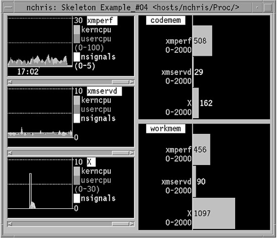
Instantiated Skeleton Console
Skeleton of Type "All"
The skeleton type named "All" includes all value
instances you select into the instrument. A skeleton
instrument creates exactly one instance of an instrument and
this single instrument contains values for all selected value
instances. This is shown in the right side of the
instantiated skeleton console shown in the preceding figure,
Instantiated Skeleton Console
. Two type "All" instruments
are defined in
the right side of the console and three processes were
selected to instantiate the skeleton console.
Skeleton instruments of type "All" are defined
with only one value because the instantiated instrument
contains one value for each of the selections you make from
the instance list.
Consoles can be defined with both skeleton instrument
types but any non-skeleton instrument in the same console is
ignored. The relative placement of the defined instruments is
kept unchanged. When many value instances are selected, it
can result in crowded instruments; but you can resolve this
by resizing the console. When all the skeleton instruments in
a console are type "All" skeletons, xmperf
does not automatically resize the console.
The type of instrument best suited for the type
"All" skeleton instruments is the state bar, but
other graph types may be useful if you allow colors to be
assigned to the values automatically. To do the latter,
specify the color as default when you define the
skeleton instrument.
Skeleton of Type "Each"
This skeleton type is so named because each value instance
you select creates one instance of the instrument. When you
select five value instances, each of the type
"Each" skeletons generates five instruments, one
for each value instance. This is shown in the left side of
the instantiated skeleton console shown in the Instantiated Skeleton Console
.
One type "Each" instrument is defined in the left
side of the console and three processes were selected to
instantiate the skeleton console.
Again, one console may define more than one skeleton
instrument and you can define consoles with both skeleton
instrument types while any non-skeleton instruments in the
same console are ignored. The relative placement of the
defined instrument is kept unchanged. This may give you very
small instruments when many value instances are selected, but
it's easy to resize the console. If the generated instruments
would otherwise become too small, xmperf attempts to
resize the entire console.
The types of instruments best suited for the
"Each" type skeleton instruments are the recording
instruments. This is further emphasized by the way
instruments are created from the skeleton:
- The relative horizontal placement is never changed.
- The relative vertical position defined by the
skeleton is never changed, but is subdivided into the
number of instruments to be created.
- Each created instrument has the full width of the
skeleton instrument.
- Each created instrument has a height which is the
total height of the skeleton divided by the number of
value instances selected.
Wildcard Restrictions
Wildcards must represent a section of a value path name
which is not the end point of the path. It could represent
any other part of the path, but it only makes sense if that
part may vary from time to time or between systems.
Currently, the following wildcards make sense:
CPU/*/...               Processing units
Disk/*/...              Physical disks
FS/rootvg/*/...         File systems
IP/NetIF/*/...          IP interfaces
LAN/*/...               Network (LAN) interfaces
PagSp/*/...             Page spaces
Proc/*/...              Processes
hosts/*/...             Remote hosts
Mem/Kmem/*/...          Kernel Memory Allocations
RTime/ARM/xaction/*/... ARM response time and activity
RTime/LAN/*/...         IP response time
Note: Not all wildcards are available on non-RS/6000
systems.
The file systems wildcard is one of the two current
example of path names where more than one wildcard would be
appropriate. It is not uncommon for a system to have more
than one volume group defined, in which case you need to
define an instrument for each volume group, as follows:
FS/rootvg/*/... Root volume group
FS/myvg/*/...   Private volume group
FS/yourvg/*/... Another private volume group
The other example is that of ARM response time metrics
where the higher level of wildcard is the application
identifier and the lower is the transaction identifier.
The xmperf program does not allow you to specify
multiple wildcards in a skeleton instrument. However, it is
possible to use dual wildcards in the 3dmon program as
described in 3D
Monitor .
When a console contains skeleton instruments, all such
instruments must use the same wildcard. Mixing wildcards
would complicate the selection process beyond the reasonable
and the resulting graphical display would be
incomprehensible.
Value Name Display
When all values in an instrument have all or part of the
value path name in common, xmperf removes the common
part of the name from the value names displayed in the
instrument and displays the common part in a suitable place.
To determine how to do this, xmperf examines the names
of all values in the containing console.
To illustrate, assume we have a single instrument in a
console, and that this instrument contains the values:
hosts/birte/PagSp/paging00/%free
hosts/birte/PagSp/hd6/%free
Names are checked as follows:
- It is checked whether all values in a console have
any of the beginning of the path name in
common. In our case, all values in the console have
the part hosts/birte/PagSp/ in common. Since
this string is common for all instruments in the
console it can conveniently be moved to the title bar
of the window containing the console. It is displayed
after the name of the console and enclosed in angle
brackets like this:
<hosts/birte/PagSp/>
The parts of the value names left to be displayed
in the instrument are:
paging00/%free
hd6/%free
- Next, each instrument in the console is checked to
see if all the value names of the instrument have a
common ending. In our example, this is the
case, since both value names end in /%free
.
Consequently, The part of the value names to be
displayed in the color of the values is reduced to:
paging00
hd6
The common part of the value name (without the
separating slash) is displayed within the instrument
in reverse video, using the background and foreground
colors of the instrument. The actual place used to
display the common part depends on the primary graph
type of the instrument.
An example of this way to display value path names
is shown in the figure Instantiated
Skeleton Console ,
where the center
instrument on the left contains the values:
hosts/nchris/Proc/4569~xmservd/kerncpu
hosts/nchris/Proc/4569~xmservd/usercpu
hosts/nchris/Proc/4569~xmservd/nsignals
The process number (4569) is not shown in the
instrument because the instrument was configured to
only show the name of the executing program.
- The last type of checking for common parts of the
value names is only carried out if the end of
the names do not have a common part. Using our
example, no such checking would be done. When
checking is done, it goes like this:
If the
beginning of the value names in an instrument (after
having been truncated using the checking described in
step 1) have a common part, this string is removed
from the value path names and displayed in reverse
video within the instrument.
To illustrate, assume we have a console with two
instruments. The first instrument has the values:
hosts/umbra/Mem/Virt/pagein
hosts/umbra/Mem/Virt/pageout
while the second instrument has:
hosts/umbra/Mem/Real/%comp
hosts/umbra/Mem/Real/%free
The result of applying the three rules to detect common
parts of the value names would cause the title bar of the
console window to display <hosts/umbra/Mem/>.
The first instrument would then have the text Virt
displayed in reverse video and the value names reduced to:
pagein
pageout
The second instrument would display Real in reverse
video and use the value names:
%comp
%free
An example of the above can be seen in the Sample xmperf Console
figure
.
The console shown in the figure has three instruments and the
values for each instrument come from the same contexts. The
path names of the three instruments (clockwise from the top
left) are:
hosts/nchris/Mem/Real/%free
hosts/nchris/Mem/Real/%comp
hosts/nchris/Mem/Real/%noncomp
hosts/nchris/CPU/cpu0/kern
hosts/nchris/CPU/cpu0/user
hosts/nchris/CPU/cpu0/wait
hosts/nchris/CPU/cpu0/idle
hosts/nchris/Mem/Virt/pagein
hosts/nchris/Mem/Virt/pageout
Hints and Tips for Using Instruments
Certain operations you can perform on an xmperf
instrument, even legal operations, can produce surprising
results. Here are a few of the things that may surprise you:
- Changing primary style
- It is quite easy to change the primary style of an
instrument. However, if you change the primary style
from a recording graph to a state graph, the
secondary style for all values are changed to that of
the new primary style. If you later want to change
the instrument back to its original style, then any
special secondary styles are forgotten.
Similarly,
secondary style information can be lost if you change
from one recording graph style to another. For
example, assume an instrument has a primary style of
bar graph, three values using this primary style, and
a single value using a secondary style, which is line
graph. If you change this instrument's primary style
to be line graph, then you lose the information about
secondary style. Had you changed the primary style to
skyline, then the secondary style would be
remembered.
- History and Shifting
- The amount of memory used to retain an image of a
recording graph is very dependent on the size of the
history and shifting properties of an instrument. In
addition, some versions of the X Window System have a
restriction that allows no pixmap (image) to be
larger than the largest window that fits on the
display. You can easily request the creation of
larger pixmaps, simply by increasing the history or
shifting properties.
If the product (history x
shift) is too large, the graph is distorted. The only
way you can currently change that is to reduce one or
both properties.
- Resizing and Moving
Instruments
- When you move or resize an instrument, you see a
rubber-band outline of the instrument until you
release the mouse button. When you move or resize the
instrument so that it overlaps other instruments, the
instrument you moved or resized is clipped so as to
prevent overlapping instruments. Only when the
clipping would result in the window being reduced to
less than 6 percent of one of the console's
dimensions is the resizing or moving terminated and
the instrument reverted to its original size and
location.
-
- Choosing Colors
- Whenever you change the color of a value or of the
foreground or background of an instrument, you see a
palette of available colors pop up on the display.
This palette may obscure the instrument where you
want to change a color.
Don't let this bother you;
simply grab the palette window and move it to the
side.To move the palette window out of the way, click
the mouse button on the title menu bar of the palette
window and hold the button down as you reposition the
window.
Notice that as you choose a color, the instrument
is changed immediately. This allows you to experiment
with colors without making permanent changes to the
instrument. When you have selected the color you
want, click on the Proceed button to make the
change permanent.
- Using Skeleton
Instruments
- When a configuration file is created on one system
and does not make use of skeleton instruments,
differences in machine hardware may make this
configuration file less useful on other systems. By
using skeleton instruments to make up for such
differences, standardized configuration files can be
designed and moved between systems.
Some common
wildcards are those represented by physical or
logical disks, page space on disks, network
interfaces, processes, and remote hosts.
- Ghost Instruments
- A console designed for one system may contain
instruments to monitor values that are not available
on another system. If the configuration file for the
first system is moved to the second system, and the
console is opened, you see empty space in the console
where the instrument used to be. The empty space
represents what is referred to as a ghost
instrument.
Ghost instruments occupy the space
and prevent you from defining a new instrument in
that same space and moving or resizing other
instruments to use the space. While this is
inconvenient, it serves the purpose of maintaining
the console definition intact if you modify other
parts of the console. Ghost instruments can not be
removed except by editing the xmperf
configuration file.
- Very Small Instruments
- If you resize a console so that a recording
instrument becomes so small that there is no space in
the instrument to draw the graph, graph data may be
written into the field at the bottom of the graph
normally reserved for time stamps. The data collected
in the history buffer is still correct. To correct
the display, resize the console to make the
instruments large enough to allow graph data to be
drawn.
Consoles
Consoles, like instruments, are rectangular areas on a
graphical display. They are created in top-level windows of
the OSF/Motif ApplicationShell class, which means that
if you use the mwm window manager, each console has
full OSF/Motif window manager decorations. These window
decorations allow you to use the mwm window manager
functions to resize, move, minimize, maximize, and close the
console.
Managing Consoles
Consoles are useful for managing instruments:
- You can move collections of instruments around in
consoles, using the console as a convenient
container.
- You can resize a console and still retain the
relative size and position of the instruments it
contains.
- You can minimize a group of instruments so that
historic data is collected and recording of incoming
data continues even when the console is not visible.
This also helps to minimize the load on your system.
- You can close a console and free all memory
structures allocated to the console, including the
historic data. Closed consoles use no system
resources other than memory to hold the definition of
the console.
Consoles can contain non-skeleton instruments or skeleton
instruments but not both. Consequently, it makes sense to
classify consoles as either non-skeleton or skeleton
consoles.
Non-skeleton Consoles
Non-skeleton consoles can be in either an opened or closed
state. You open a console by selecting it from the Monitor
menu. Once the console has been opened, it can be minimized,
moved, maximized, and resized using mwm. None of these
actions change the status of the console. You might not see
the console on the display, but it is still considered open
and if recording has been started, it continues.
If you look at the Monitor menu after you have opened one
or more non-skeleton consoles, the name of the console is now
preceded by an asterisk. This indicates that the console is
open. If you click on one of the names preceded by an
asterisk, you close the corresponding console.
Skeleton Consoles
Skeleton consoles themselves can never be opened. When you
select one from the Monitor menu, you are presented with a
list of names matching the wildcard in the value names for
the instruments in the skeleton console. If you select one or
more from this list, a new non-skeleton console is created
and added to the Monitor menu. This new non-skeleton console
is automatically opened, and given a name constructed from
the skeleton console name suffixed with a sequence number.
The non-skeleton console created from the skeleton is said
to be an "instance" of the skeleton console; we say
that a non-skeleton console has been instantiated from
the skeleton. The instantiated non-skeleton console works
exactly as any other non-skeleton console, except that
changes you make to it never affect the configuration file.
You can close the new console and reopen it as often as you
wish, and you can resize, move, minimize, and maximize it.
Each time you select a skeleton console from the Monitor
menu you get a new instantiation, each one with a unique
name. For each instantiation you'll be prompted to select
values for the wildcard, so each instantiation can be
different from all others.
If you have created an instance of a skeleton console and
you'd like to change it into a non-skeleton console and save
it in the configuration file, the easiest way to do so is to
choose Copy Console from the Console menu. This
prompts you for a name of the new console and the copy is a
non-skeleton console that looks exactly like the instantiated
skeleton console from which you copied. Once you have copied
the console, you can delete the instantiated skeleton console
and save the changes in the configuration file.
Placing Instruments in Consoles
Within their enclosing ApplicationShell windows,
all consoles are defined as OSF/Motif widgets of the XmForm
class and the placement of instruments within this container
widget is done as relative positioning. Relative positioning
has advantages and disadvantages. One advantage is the easy
resizing of a console without loss of relative positions of
the enclosed instruments. A disadvantage is the complexity
involved when adding or removing an instrument in an already
full console.
Adding an Instrument to a Console
When you want to add an instrument to a console, you can
choose between adding a new instrument or copying one that's
already in the console. If you choose to create a new
instrument, the following happens:
- It is checked if there is enough space to create an
instrument with a height that is approximately the
average height of any existing instruments in the
console. If no instruments exist, the height is set
to 25% of the console. The space must be available in
the entire width of the console. If this is the case,
a new instrument is created in the space available.
- If enough space is not available, the existing
instruments in the console are resized to provide
space for the new instrument. Then the new instrument
is created at the bottom of the console. The height
of the new instrument will be approximately the
average height of any existing instruments, after
resizing.
- If the new instrument has a height less than 100
pixels, the console is resized to allow the new
instrument to be 100 pixels high.
If you choose to copy an existing instrument, the
following happens:
- It is checked if there is enough space to create an
instrument of the same size as the one you copy. If
this is the case, a new instrument is created in the
space available. Unlike what happens when adding a
new instrument, copying will use space that is just
wide enough to contain the new instrument. There's no
need to have space available in the full console
width.
- If enough space is not available, the existing
instruments in the console are resized to provide
space for the new instrument. Then the new instrument
is created. New space is always created at the bottom
of the console, and always in the full width of the
console window. However, the new instrument will have
the same width as the one it is a copy of.
- If the new instrument has a height less than 100
pixels, the console is resized to allow the new
instrument to be 100 pixels high.
Rounding may cause the height of the new instrument to
deviate 1-2 percent from the intended height.
Resizing Instruments in a Console
Once you've selected an instrument and chosen to resize
it, the instrument goes away and is replaced by a rubber-band
outline of the instrument. You resize the instrument by
holding mouse button 1 down and moving the mouse. When you
press the button the pointer is moved to the lower right
corner of the outline and resizing is always done by moving
this corner while the upper left corner of the outline stays
where it is.
During resizing, a small button is shown in the top left
corner of the rubberband outline. It shows the calculated
relative size of the instrument as width x height in percent
of the console's total width and height. The relative size is
calculated from the relative positions of the edges of the
instrument as:
- width = right_edge - left_edge + 1
- height = bottom_edge - top_edge + 1
For example, for an instrument to have a width of 49 and a
height of 20, the edges might have the following relative
positions:
- top_edge = 20
- left_edge = 1
- right_edge = 49
- bottom_edge = 39
When you release the mouse button the instrument is
redrawn in its new size.
Note that it's normally a good idea to move the instrument
within the console so that the upper left corner is at the
desired position before resizing.
The position of the resized instrument must be rounded so
that it can be expressed in percentage of the console size.
This can cause the instrument to change size slightly from
what the rubber-band outline showed.
Instruments can not be resized so they overlap other
instruments. If this is attempted, the size is reduced so as
to eliminate the overlap.
Moving Instruments in a Console
When you select an instrument to be moved, the instrument
disappears and is replaced by a rubber-band outline of the
instrument. To begin moving the instrument, place the mouse
cursor within the outline and press the left mouse button.
Hold the button down while moving the mouse until the outline
is where you want it, then release the button to redraw the
instrument.
During moving, a small button is shown in the bottom right
corner of the rubberband outline. It shows the calculated
relative position of the top left corner of the instrument.
This helps in positioning the instrument so that it aligns
with the other instruments in the console.
Instruments can be moved over other instruments, but are
not allowed to overlap them when the mouse button is
released. If an overlap would occur, the instrument is
truncated to eliminate the overlap.
The Console Title Bar
The title bar of a console window contains three pieces of
information. It might look like this, for example:
birte: Virtual Memory <hosts/xtra/Mem/Virt/>
The first two pieces of information are always present.
The third part is only displayed if all statistics displayed
in the console's instruments have some or all of the
beginning of their value names in common. The three parts of
the title bar text are:
- The hostname of the system where xmperf is
executing. It is followed by a colon to separate it
from the next part of the text.
- The name of the console. In case of instances of
skeleton consoles, the name might look like this:
Disks_#01
where the name of the skeleton console would then
be Disks and the remainder is added to give
the instantiated skeleton console a unique name.
- Any common part of all values displayed in the
console enclosed in angle brackets. For a description
of how this part is generated, see Value Name Display
.
When
values are added to or removed from the console, the
common part of the value names might change. When
this happens, the console title bar changes to
reflect this.
Environments
Environments are defined in configuration files. By
default, xmperf reads its environment from the file
$HOME/xmperf.cf
or, if that file does not exist, then as described in
File Placement Overview
.
You can override the file name through the command line
argument -o or the X Window System resource ConfigFile.
Command line arguments are described in
The xmperf Command Line
and supported resources in The
xmperf Resource File section .
In most situations, any one person should be able to stick
to a single environment, defining all the consoles required
for the monitoring that person needs. However, since the
environment holds not only console definitions but also
command definitions as described in The xmperf Command Menu Interface
,
different environments can be defined for different kinds of
users. Most of all, this is a matter of what privilege is
required to execute the commands.
A system administrator may be authorized to run commands
such as renice and other commands that require root
authority. Therefore, the system administrator may want to
have more commands or different ones. When xmperf uses
such environments, it can be necessary to start the program
while logged in as root.
Monitoring Remote Systems with
xmperf
Note: This function is only available with the
Performance Toolbox Network feature. If you try to access
these functions with the Performance Toolbox Local
feature only the local hostname is displayed for
selection.
Visualizing the load statistics (or monitoring the
performance) of a single local host on that same host has
been done with a great variety of tools, developed over many
years. The tools can be useful for critical hosts such as
database servers and file servers, provided you can get
access to the host and that the host has capacity to run the
tool.
Some of the existing tools, especially when based on the X
Window System, allow the actual display of output to take
place on another host. Even so, most existing tools depend on
the full monitoring program to run on the host to be
monitored, no matter where the output is shown. This induces
an overhead from the monitoring program on the host to be
monitored.
Performance Toolbox for AIX introduces true remote
monitoring by reducing the executable program on the system
to be monitored to the Agent component's xmservd
program, which consists of a data retrieval part and a
network interface. It is implemented as a daemon that is
started by the inetd super-daemon when requests from
data consumers are received. The xmservd program is
described in Monitoring
Remote Systems .
The obvious advantage of using a daemon is that it
minimizes the impact of the monitoring software on the system
to be monitored and reduces the amount of network traffic.
Because one host can monitor many remote hosts, larger
installations may want to use dedicated hosts to monitor many
or all other hosts in a network.
The responsibility for supplying data is separated from
that of consuming data. Therefore, we have adopted the term
data-supplier host to describe a host that supplies
statistics to another host, while a host receiving,
processing, and displaying the statistics is called a
data-consumer host.
The Meaning of Localhost in xmperf
All data-consumer programs made to the RSi API (see
RSi Programming Guide),
such as xmperf, are always doing remote monitoring in
the sense that they can get their flow of statistics only
from data supplier daemons. It is immaterial to the protocol,
as to the programs, whether the daemon feeding a particular
instrument runs on the local or a remote host.
It is, however, convenient that you can create and
maintain consoles for the local host. The term Localhost
refers to the host that all instruments in the xmperf
configuration file are assumed to refer to when no hostname
is given as part of their value path names.
The Localhost defaults to the host where xmperf
is executing. Any other host can be selected at the time you
start xmperf, using the command line argument -h.
The Localhost can not be changed while xmperf
is running.
Note: A change of Localhost has no
influence on where commands, defined in the main window
pulldown menus, are executed. Commands are always
executed on the host where xmperf runs.
When to Identify Data-Suppliers
The xmperf program attempts to contact potential
suppliers of remote statistics in the following situations:
- When the program starts, it always attempts to
identify potential Data-Supplier hosts.
- When five minutes have passed since the last attempt
to contact potential data-supplier hosts and the user
creates an instrument referencing a remote
data-supplier host.
- When five minutes have passed since the last attempt
to contact potential data-supplier hosts and the user
activates a console containing a remote instrument.
- When five minutes have passed since the last attempt
to contact potential data-supplier hosts and the user
requests the Remote Process Window from the
xmperf Utilities menu.
- When the user selects the Refresh Host List
entry from the xmperf File menu.
The five-minute limit is implemented to make sure that the
data-consumer host has an updated list of potential
data-supplier hosts. Please note that this is not an
unconditional broadcast every five minutes. Rather, the
attempt to identify data-supplier hosts is restricted to
times where a user wants to initiate remote monitoring and
more than five minutes have elapsed since this was last done.
The five-minute limit not only gets information about
potential data-supplier hosts that have recently started; it
also removes from the list of data suppliers such hosts,
which are no longer available. In heavily loaded networks and
situations where one or more remote hosts are too busy to
respond to invitations immediately, the refresh process may
remove hosts from the list even though they do in fact run
the xmservd daemon. If this happens, you should use
the -r command line argument when you invoke xmperf.
Through this option, you can increase the time xmperf
waits for remote hosts to respond to invitations.
How Data-Suppliers are Identified
Once xmperf is aware of the need to identify
potential data-supplier hosts, it uses one or more of the
following methods to obtain the network address for sending
an invitational are_you_there message. For a full
description of network packet types and the network protocol
see The xmquery
Network Protocol
. The last two methods depend on the
presence of the file $HOME/Rsi.hosts
. See
Overview of File Placement
,
for alternative locations of the Rsi.hosts
file.
The three ways to invite data-supplier hosts are:
- Unless instructed not to by you, xmperf finds
the broadcast address corresponding to each of the
network interfaces of the host where xmperf is
executing. The invitational message is sent on each
network interface using the corresponding broadcast
address. Broadcasts are not attempted on the
Localhost (loopback) interface or on point-to-point
interfaces such as X.25 or SLIP (Serial Line
Interface Protocol) connections.
- If a list of Internet broadcast addresses is supplied
in the file $HOME/Rsi.hosts
, an
invitational message is sent on each such broadcast
address. Every Internet address given in the file is
assumed to be a broadcast address if its last
component is the number 255. Note that if you specify
the broadcast address of a local interface,
broadcasts are sent twice on those interfaces. In
large networks, this may produce an unacceptably
large number of response to invitational packets.
- If a list of hostnames or non-broadcast Internet
addresses is supplied in the file $HOME/Rsi.hosts
,
the host Internet address for each host in the list
is looked up and a message is sent to each host. The
look-up is done through a gethostbyname()
call, so that whichever name service is active for
the host where xmperf runs is used to find the
host address. If your nameserver is remote or often
slow to respond, specify Internet addresses rather
than hostnames to avoid the delay caused by the name
lookup.
The file $HOME/Rsi.hosts
has a very simple
layout. Only one keyword is recognized and only if placed in
column one of a line. That keyword is:
nobroadcast
and means that the are_you_there message should not
be broadcast using method 1 (where an invitation is sent to
the broadcast address of each network interface on the host).
This keyword is useful in situations where there is a large
number of hosts on the network and only a well-defined subset
should be remotely monitored. To say that you don't want
broadcasts but want direct contact to three hosts, your
$HOME/Rsi.hosts
file might look like this:
nobroadcast
birte.austin.ibm.com
gatea.almaden.ibm.com
umbra
The previous example shows that the hosts to monitor do
not necessarily have to be in the same domain or on a local
network. However, doing remote monitoring across a low-speed
communications line is not likely to make you popular with
other users of that communication line.
Be aware that whenever you want to monitor remote hosts
that are not on the same subnet as the data-consumer host,
you must specify the broadcast address of the other subnets
or all the host names of those hosts in the $HOME/Rsi.hosts
file. The reason is that IP broadcasts do not propagate
through IP routers or gateways.
Note: Other routers can be configured to
disallow UDP broadcast between subnets. If your routers
disallow UDP broadcasts, enter the Internet address or
hostname of all the hosts you want to monitor on other
subnets in the $HOME/Rsi.hosts
file.
The following example illustrates a situation where you
want to do broadcasting on all local interfaces, want to
broadcast on the subnet identified by the broadcast address
129.49.143.255, and also want to invite the host called umbra.
129.49.143.255
umbra
Note: The subnet mask corresponding to the
broadcast address in this example is 255.255.240.0 and
the range of addresses covered by the broadcast address
is 129.49.128.0 through 129.49.143.255.
Requesting Exception Messages
One of the message types passing between dynamic
data-supplier and data-consumer hosts has a field that is
used to tell the responding xmservd daemons whether
any exception notifications (actually network packets of type
except_rec) they may generate should be sent to the
data-consumer host. Application programs control this field
through the last argument to the
RSiOpen
and
RSiInvite
subroutine calls of the Remote Statistics Interface API. By
default, the xmperf program does not request exception
messages to be sent to it. This can be controlled through the
command line argument -x or the X resource GetExceptions.
Exception messages are used to inform about abnormal
conditions detected on a system. They are described in the
Handling Exceptions
.
When xmperf receives an exception message, it is
displayed in the xmperf main window. No other action
is taken. A better way of monitoring exceptions is provided
by the program exmon described in the
Monitoring Exceptions
with exmon .
Remote Processes
Two of the three main window menus that are used to define
command menus have a fixed menu item. Those main window menus
are Controls and Utilities. This section describes the Remote
Processes fixed menu item in the Utilities pulldown menu.
The purpose of the Remote Processes menu item is to provide
you with an easy way to display the CPU-intensive processes
on a remote host, which runs the xmservd daemon.
If you are monitoring remote systems you'll recognize the
need for this function. It is not uncommon that a console
used to monitor a remote host suddenly shows that something
unexpected or unusual is happening on the host. To see what
causes this, you would need to look into the processes that
run on the remote host. However, it takes time to do a remote
login and may even be impossible for certain types of errors
or certain types of loads. This menu allows you to list key
data for all processes running on the remote host without the
need to do a remote login.
The first thing that happens when you select Remote
Processes is that you see a list of remote hosts from
which to select. An example of such a selection list is shown
in the following figure, Host Selection List from xmperf
.
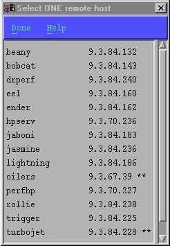
Host Selection List from xmperf
Remote Process List
When you select a host to monitor from Remote Processes,
you immediately see a list of running processes in the remote
host at the time you made the selection. It depends on the
currently active display option (see Remote
Processes Menu
for details of how to set this
option) of the remote process list whether all the processes
of the remote host are shown, or whether only CPU-active
processes are included. The list shows the most interesting
details about the processes, and is sorted in descending
order according to the CPU percentage used by the process. An
example of a remote process list is shown in the following figure,
Remote Process List from xmperf
.
Remote Process List from xmperf
The fields in the list are,
from left to right:
- Host path
- The path used to get to the remote host in the form
hosts/hostname.
- Command Name
- The text "Process" followed by the (first 9
bytes of) the command that executes in the process.
- Process ID
- The process ID (PID) of the process.
- Latest CPU Percentage
- The first time the remote process list is created
after the start of the xmservd daemon on the
remote host, this field shows the CPU usage of the
process over its life time. The same is true whenever
a new process shows up on the process list after a
refresh. In all other cases, this field shows the
average CPU usage since the last refresh of the
process list.
- Page Space in
Megabytes
- The number of megabytes currently allocated for
paging space on an external disk for this process.
- Effect User-ID
- The effective user ID for the process, as changed by setuid
or su if applicable.
Note: The fields shown in remote
process lists for non-RS/6000 systems may
vary from the fields shown here.
Remote Processes Menu
When the process overview list is displayed, a menu bar is
available to control the list. The following menu items are
available:
- File
- This menu item yields a pulldown menu with four menu
items:
- Refresh
- Refreshes the list by reading the current process
information from the daemon on the remote host.
- Show All
- Changes the display option of the remote process
list so that all processes of the remote host are
shown, regardless of their CPU usage.
- Show CPU Active
- Changes the display option of the remote process
list so that only processes of the remote host
that have been using CPU since the last refresh
are shown.
- Close
- Closes the list.
- Help
- Displays any help text supplied in the simple help
file and identified by the name Remote Process
List
.
Note: The
process list is not updated by xmperf
automatically. It is your responsibility to use
the Refresh menu item to have the list
updated as needed. It is updated whenever you
change the display option.
[ Previous |
Next |
Contents |
Glossary |
Search ]