Structures are defined in the centralized structure store, independent of any workstation. Your application has two types of facilities to display the graphical data in structures:
This chapter discusses the functions that give your application control over whether its graphic data is associated with or disassociated from views and workstations and the way the graPHIGS API processes a root's structure network. It is essential that you understand this process in order to conceptualize how to achieve desired results on a display device.
This section discusses how to associate portions of graphics data with a workstation or workstations, and make it eligible for display. When your application associates a structure with a workstation or a view, that structure becomes known as a root structure.
In the sample program introduced in Chapter 1, the statements:
       CALL GPASSW(WSID,1)
       CALL GPARV(WSID,VIEW1,STRID(1),1.0)
first associates structure store 1 to all views of the workstation, then structure 1 (the root structure) is associated with view 1 of the workstation enabling your application to display the house on your graphics terminal. A detailed discussion of structure stores is contained in Part Two of this manual.
The graPHIGS API splits the process of associating roots into two program subroutine calls that let your application separately associate a root with a workstation and with a view. This lets your application take advantage of intelligent workstations that can store graphics data even when it is not needed for display. For example, your application may choose to store many menus at a workstation of which only one is displayed at a time. Another menu can then be displayed quickly by associating the structure to a view, in which case only the association data (and not the entire menu structure) needs to be sent to the workstation. The figure, "Workstation Capable of Storing Associated and Non-Associated Structures," depicts a workstation's storage in which stored structures are both associated and not associated with views.
The Associate Root with a Workstation (GPARW) subroutine lets your application associate a structure network with a workstation. This lets your application pre-load structures that may be required later.
When the data resides at the workstation, your application only needs to associate these structures to a view for display. This reduces communication time, and provides better response time, since at the display time, only the root identification information is sent, not the graphics data.
The Associate Root With View (GPARV) subroutine lets your application associate a structure network, with a view and, implicitly, a workstation. It also lets your application specify the priority of the root structures within that view.
Similar to the priority of views, the graPHIGS API processes root structures within each view in reverse priority order. This results in higher priority networks overlaying lower priority networks on the display surface. This gives your application the following three ways of controlling display priority:
The graPHIGS API provides program subroutine calls that let your application alter the relationships between structure networks, views, and workstations. None of the subroutine calls in this section delete a root structure network from the centralized structure storage. They only modify the relationship between the root and the specified workstation.
The Disassociate Root from Workstation (GPDRW) subroutine lets your application remove a specified structure from a specified workstation. The GPDRW subroutine is the logical reverse of the Associate Root With Workstation (GPARW) subroutine. If the structure is no longer referenced by any other structure on this workstation, the API removes that structure from the workstation. It also removes all of its sub-structures if those sub-structures do not belong to another root's network. The GPDRW also removes that structure from all views.
The Disassociate All Roots from Workstation (GPDARW) subroutine lets your application remove all structures from a specified workstation. Upon completion of the GPDARW suboutine, the workstation's list of associated roots is empty. Thus, it also empties all views.
The Disassociate Root from View (GPDRV) subroutine lets your application remove a specified root from a view on a specified workstation. The root remains associated with the workstation. The GPDRV is the logical reverse of the associate root with view (GPARV) subroutine.
The Disassociate Root from All Views (GPDRAV) subroutine lets your application remove a specified root from all views on a given workstation.
The Empty View ( GPEV) subroutine lets your application remove all the roots from a specified view. Upon completion of the GPEV subroutine, the specified view exists but displays no graphics data.
The Empty All Views (GPEAV) subroutine lets your application remove all the roots from all the views at a specified workstation.
After associating structure networks with views and workstations, your application can initiate the process of displaying an image on an output device. This process involves a sequential traversal of the structure elements.
In the sample program introduced in Chapter 1, after associating the structure to the workstation and view, the statement:
CALL GPUPWS(WSID,2)
initiates the structure traversal process and generates the house drawing on the workstation display.
As shown in the figure, "Structure Traversal Processing," each view is traversed in the order of its assigned priority, from lowest to highest. Within each view, root structures and their corresponding networks are likewise processed in reverse priority order. Therefore, structure traversal begins by processing the lowest priority root structure in the lowest priority view.
Each time the traversal of a root's structure network is initiated, a default set of attribute and transformation values exists in a conceptual set of traversal-time registers. For example, the default composite modeling transformation matrix is the identity matrix, and the default line type is 1=SOLID_LINE. The complete set of traversal-time default values can be found in The graPHIGS Programming Interface: Technical Reference
Structure elements which set attributes or define modeling transformations may modify these conceptual registers. Other structure elements of the same structure, or of another structure invoked by this same structure, may use the values in these conceptual registers.
The traversal of a root's structure network begins at element one of the root structure. Elements are then processed sequentially, ending with the last element of the root structure. After completing the processing of a root structure, the API proceeds to traverse either the root with the next highest priority, or if this was the last root in the current view, it continues to the next highest priority view. The traversal process ends when the highest priority view is completely traversed.
As the graPHIGS API processes the structure networks, it encounters elements sequentially. As it encounters these elements, the effect of processing a given element results in one of the following four actions:
Each time the graPHIGS API encounters an output primitive, it applies the current attribute and transformation values to that primitive. The current values reflect changes that are due to structure element assignments or inheritance. This is called traversal-time attribute binding
Barring any local attribute assignments, when a primitive is referenced by multiple structures, the appearance of that primitive is determined, in each instance, by the inherited attributes.
When encountering a GPEXST element within a structure, the system suspends traversal of that structure. It also saves the current transformation and attribute values. Then it completely traverses the invoked structure. On return to the structure, the API restores the state of the transformation and attribute values, then resumes structure traversal.
During structure traversal, the system keeps track of the current attribute values in the traversal-time registers. When encountering an output primitive, the system checks the ASF setting of each attribute to determine whether it obtains that attribute from the system's conceptual attribute registers, or from a workstation's bundle table. These conceptual registers contain either an attribute specification or an index into a bundle table.
The current values can consist of default values, inherited values, and assigned values as a result of any attribute assignment element.
Each time the system encounters an output primitive, it passes that primitive's coordinate data through a series of transformations before displaying output on a device. This series of transformations is called the transformation pipeline depicted in the figure, "Transformation Pipeline With Relation to the Various Coordinate Systems."
The treatment of this subject is done here at a conceptual level. How the implementation actually realizes the capabilities described here may be significantly different from the conceptual, stepwise process described here. For example, an intelligent workstation may be able to collapse consecutive transformations into only one transformation. Most important to the application programmer is that the system always functions identical to this conceptual description.
Data does not pass through the pipeline until it is time to display the data.
The transformation pipeline begins with the coordinate system within which your application defines its graphics data, the Modeling Coordinate System (MCS). The pipeline ends with the Device Coordinate System (DCS), which provides the coordinates used by the output workstation hardware.
The pipeline consists of five distinct coordinate systems with four transformation processes which transform that data from the MCS to the DCS.
In the trivial case, a step in the pipeline is equal to an identity transformation. An identity transformation is the system's default for both modeling and viewing transformations. In this case, the transform does not affect the data in any way.
Only the modeling transformations can be modified by structure elements during structure traversal. All other transformations are set by way of control subroutines that are contained in tables. With the exception of the modeling transformation value, all transformation values are established when structure display traversal is initiated. The following sections discuss the function of each step in the transformation pipeline.
The graPHIGS API defines all primitives in the Modeling Coordinate System (MCS). Your application may use any portion of modeling space. Modeling space is only bounded by the range representable by a 32-bit real number.
A typical usage is to define primitives in different portions of modeling space and then "assemble" them to create the final model. The "assembling" of parts of the model is done using modeling transformations. They transform the primitive's coordinates into a common coordinate system called the World Coordinate System (WCS).
Modeling transformations modify the coordinates of a primitive in an application-defined manner. The modeling transformation (like all transformations) is represented by a 4 [default] 4 matrix. Modeling transformations may translate the data, scale the data, rotate the data, or any other operation possible by the multiplication of a coordinate by a 4 [default] 4 matrix. The default modeling transformation is an identity transformation.
After the modeling transformation is applied, all data is in the World Coordinate System (WCS). Like modeling space, world coordinate space is only bounded by the range representable by single precision floating-point numbers.
When your application defines a view it indicates to the system what portion of the World Coordinate System it wants to display.
By means of the viewing transformation, world coordinate data is transformed into the Viewing Coordinate System. Your application can use the viewing transform to rotate, scale, or in some way modify the world coordinate data and transform it into the Viewing Coordinate System.
Any combination of structures may be viewed using the same view definition. Your application can use a structure in many views. More than one view may exist for each workstation and their definitions are contained in the view table. There is one view table for each workstation.
It is from the viewing coordinate system that the projection operation takes place. The type of projection (or view) of the data may be parallel or perspective. The region to be projected is defined by two clip planes, a window, a projection reference point (eye point), a view plane position (for projecting onto) and a projection type.
After the data is projected it is mapped, by way of the defined view mapping, into the Normalized Projection Coordinate (NPC) system. The view mapping consists of a window on the view plane near/far clip planes and a viewport in NPC space.
As the name implies, NPC space is a normalized coordinate system. NPC extends from 0.0 to 1.0 in the X, Y and Z directions. A viewport, in this space, is defined as minimum and maximum X, Y and Z values which define a viewport volume in NPC space.
The final step in the transformation of the data to the display takes the data from NPC space to the coordinate system of the device. The workstation transformation takes the data from NPC to Device Coordinates (DC). There is one workstation transformation per workstation. The workstation transform positions the logical workstation's display surface on the physical display. In the default case, all of NPC is mapped onto all of DC. Most applications do not modify this relationship.
Device Coordinates (DC) are typically defined in meters and express the actual size of the physical display. Another means of describing the display characteristics is address units (rasters) which measure the actual addressability of the display. Both the address units and device coordinates used by a workstation may be determined by inquiries.
There are two methods the graPHIGS API uses to display data in an X-Window: 1=MAPPED and 2=DIRECT Use the Set Device Coordinate Mapping Method (GPDCMM) subroutine to choose the method that best suits your application.
By default, the graPHIGS API uses the 1=MAPPED display method. This method displays data in an X-Window by scaling the graPHIGS API device coordinate (DC) range to fit the X-Window. When you change the X-Window size, the graPHIGS API scales the contents to fit the new window. In this way the aspect ratio of the data is preserved, the same amount of data is displayed regardless of scale, and the window can be said to behave like a "rubber sheet"
When using the DIRECT method, the graPHIGS API displays the DC range directly in the X-Window with no scaling. The lower-left corner of the DC volume is aligned with the lower-left corner of the window. If the window is smaller than the DC range addressed in the data, then the window clips the data. If the window is larger than the display data, the area of the window beyond the DC range of the data is unused. This window behavior can be likened to that of a "porthole"
Refer to The graPHIGS Programming Interface: Technical Reference for more information on the 2=DIRECT method of display in an X-Window.
During structure traversal, the system keeps track of the current global and local modeling transformation matrixes in conceptual registers. When root structure traversal begins, the default matrix for both the global and local matrixes is the identity matrix.
During structure traversal, each substructure inherits only one composite transformation matrix. The composite matrix is the concatenation of the local modeling transformation and the global transformation at the time the GPEXST element is encountered. The graPHIGS API refers to the composite matrix in the parent structure as the global modeling transformation matrix of the invoked structure. The figure, "How Structures Inherit Transformation Matrixes," depicts how structures beginning with the tabletop structure inherit transformation matrixes:
When encountering the tabletop primitive, the system multiplies the tabletop's Modeling Coordinates (MC) by the concatenation of L2 and G1.
When encountering the leg primitive, the system multiplies the leg's coordinates by the concatenation of the appropriate inherited matrix and the leg's local modeling transformations. Notice that L3 through L6 all use the replace concatenation type option. As discussed in Chapter 3. "Structures", the concatenation type option specifies how the modeling transformation element operates on the current modeling transformation values.
Drawing the first leg entails multiplying the leg's coordinates by a concatenation of L7 and G3.
Drawing the second leg entails multiplying the leg's coordinates by a concatenation of L7 and G4.
Drawing the third leg entails multiplying the leg's coordinates by a concatenation of L7 and G5.
Drawing the fourth leg entails multiplying the leg's coordinates by a concatenation of L7 and G6.
Your application may override the inherited global transformation by using the Set Global Transformation (GPGLX2 and GPGLX3) subroutine. The new global transformation matrix replaces the previous global matrix.
Primitives may be grouped by your application into application-defined classes. By using filters, provided by the graPHIGS API, your application may control the detectability, highlighting and invisibility of these primitives. During structure traversal, the system manages the current class name values and resolves which primitives are detectable, highlighted, or visible, based on the primitive's class specification.
To this end, the system supports the following three inclusion and exclusion filters:
These filters operate independently of each other. Making a particular class of primitives detectable, for example, does not affect whether that class is highlighted or visible.
To provide dynamic control over which classes are detectable, highlighted, and visible, each filter contains an inclusion filter and an exclusion filter.
These filters control the detectability, highlighting, and invisibility of entire classes of output primitives.
The system provides a consistent set of rules that govern the interrelationships between classes assigned to inclusion and exclusion filters. An output primitive is detectable, highlighted, or invisible if and only if both of the following are true:
When all of the filters are empty, for example, at initialization time:
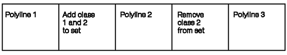
Inclusion and exclusion filter designations are control subroutine calls that modify the workstation state. The figure, "Root structure with class designations," depicts a root structure with class designations:
By proper organization of structure content, your application can modify these characteristics of primitives without structure editing. In the figure, "Root structure with class designations," polyline 1 can not be made detectable, highlighted, or invisible. Polyline 2 is affected by how your application assigns classes 1 and 2 to inclusion and exclusion filters. Polyline 3 is affected only by how your application assigns class 1 to inclusion and exclusion filters.
The Set Pick Filter (GPPKF) subroutine enables your application to specify which classes belong to a pick device's inclusion and exclusion filters. Using the information in the figure, "Root structure with class designations," an assignment of class 1 to only the pick inclusion filter, makes both polyline 2 and polyline 3 detectable.
The graPHIGS API enables your application to control the highlighting of primitives. The Set Highlighting Filter (GPHLF) subroutine enables your application to specify which classes belong to highlighting inclusion and exclusion filters. Using the information in the figure, "Root structure with class designations," if your application only assigns class 2 to the the highlighting inclusion filter, then only polyline 2 is highlighted. Because polyline 3 only belongs to class 1, it is affected only by those changes that affect class 1 because class 2 is removed before polyline 3 is drawn.
The graPHIGS API lets your application specify whether a primitive or set of primitives are visible. The Set Invisibility Filter (GPIVF) subroutine lets your application control which classes are in a workstation's inclusion and exclusion filters. Remember that the default is the absence of classes in either filter. This means that all primitives are initially visible. Using the information in the figure, "Root structure with class designations," if your application assigns class 1 to the invisibility inclusion filter and class 2 to the invisibility exclusion filter, then polyline 3 becomes invisible. In order to analyze why polyline 2 remains visible remember the rules that govern how filters affect primitives. Polyline 2 remains visible because at least one class (number 2) is in the invisibility exclusion filter. This excludes polyline 2 from becoming invisible.
The graPHIGS API provides two methods for your application to assure that the display image corresponds exactly to the state of the system.
The Redraw All Structures (GPRAST) subroutine forces a new frame action on the specified workstation, and then rebuilds the display based on the current state of the system. A new frame action involves clearing the screen on the display or feeding a new sheet of paper on a plotter-type device.
The Update Workstation (GPUPWS) subroutine assures that the display exactly matches the state of the system. A new frame action occurs only if necessary.
When GPUPWS is called, all deferred actions for the specified workstation are executed without an intermediate clearing of the display surface. If the regeneration flag is set to PERFORM and a new frame action is necessary the following actions are taken on the specified workstation:
With the Update Workstation Asynchronous (GPUPWA) subroutine, transactions with the specified workstation do not wait for an on-going traversal to complete. This means that a traversal may be interrupted before completion, causing intermediate screen changes to go unseen. (It may be important, for example in animation sequences, to see all updates to the workstation in a sequential fashion. In this case, the synchronous Update Workstation (GPUPWS) subroutine should be used. Use GPUPWA when it is necessary to see the most up-to-date screen as soon as possible).
When there are no changes pending at the workstation, and GPUPWS is called, no action occurs. On the other hand, if your application invoked GPRAST in this situation, the workstation clears the display surface and re-displays the same image. On a plotter-type device, this can be used to generate many identical plots.
Deferral modes let your application control when the graPHIGS API traverses the structure networks and generates an image on a particular workstation. The following deferral modes let your application control the deferral state of the system:
These modes do not affect when structure editing occurs, rather they affect when structure modifications are seen on the display surface. Since your application can edit structure networks without changing the output image, the image may not reflect the current graphics data within the structure networks. These deferral modes let your application control when to resolve the differences between the structure definitions and the image.
When the deferral mode is satisfied, the API traverses the structures and generates an image that corresponds to the graphics data in the structure networks and the current settings in the workstation's tables, that is, a GPUPWS is performed.
Your application may choose to defer changes to an image when a lot of editing occurs, in order to buffer the changes and optimize the transfer of data.
Remember that the GPUPWS subroutine causes an immediate traversal of the structure networks and generation of an image on an output device, no matter what deferral mode is in effect.
Deferral modes have many application-defined uses. For example, your application may choose to prevent an image change until a particular condition is satisfied.
1=ASAP Deferral Mode: When a workstation is in ASAP deferral state, the API re-traverses all data after every program subroutine call and updates the output image. This state introduces the maximum system overhead per subroutine call.
2=BNIG Deferral Mode: A workstation in BNIG mode is updated immediately before an interaction occurs at any open workstation. For example, suppose workstation one is in ASAP mode and workstation two is in BNIG mode. If an output display operator interacts with workstation one, the system updates workstation two before the interaction takes place.
Notice that when your application uses BNIG and it places an input device in Sample or Event mode, the system always re-traverses the structure networks, since on every subroutine call an interaction is always underway. Until the input device mode is changed, the BNIG mode simulates the ASAP mode. This may adversely affect performance.
3=BNIL Deferral Mode: A workstation in BNIL mode is updated immediately before an interaction occurs at that workstation.
For example, suppose that workstation one is in ASAP mode, workstation two is in BNIG mode, and workstation three is in BNIL mode. If an output display operator interacts with workstation two, then the system updates workstation one and two, but not three. However, if the display operator interacts in workstation three, then the API updates all three workstations.
Notice that when your application uses BNIL and it places an input device in sample or event mode, the system re-traverses the structure networks, since on every subroutine an interaction is always underway. Until the input device mode is changed, the BNIL state simulates the ASAP mode. This may adversely affect performance.
4=ASTI Deferral Mode: Changes to the image of a workstation in ASTI mode occur in an implementation-dependent way. This implementation treats ASTI the same as BNIL.
5=WAIT Deferral Mode: The WAIT deferral mode is the default mode. In this mode, all changes to a workstation are deferred until your application explicitly requests them. Your application can cause changes to a workstation in WAIT state by:
Notice that, in this mode, your application defers all changes to a workstation until the GPUPWS subroutine is issued.
The graPHIGS API supports three Modification Modes selectable through the Set Deferral State (GPDF) subroutine.
For information on the use of these modes, see the The graPHIGS Programming Interface: Writing Applications .
QUICK_UPDATE mode allows the graPHIGS API, running with XLIB and XDWA device drivers, to show the results of structure editing functions by direct screen modification, eliminating the need for a complete screen redraw. Use of QUICK_UPDATE should be weighed against the need for thoroughly accurate screen contents, since the results of a QUICK_UPDATE may not be perfectly displayed.
When operating in QUICK-UPDATE mode, the application performs as many structure editing operations as possible without redrawing the screen. The success of a QUICK_UPDATE depends on the target structure element and the editing operation. Class name, for example, cannot be changed using QUICK_UPDATE. When the graPHIGS API finds that an operation leaves the display too inaccurate, it terminates the QUICK_UPDATE operation and redraws the screen.
Refer to The graPHIGS Programming Interface: Technical Reference for more information on QUICK_UPDATE .