|
IBM POWER Systems Overview
|
|
Table of Contents
- Abstract
- Evolution of IBM's POWER Architectures
- Hardware Overview
- System Components
- POWER4 Processor
- POWER5 Processor
- Nodes
- Frames
- Switch Network
- GPFS Parallel File System
- LC POWER Systems
- Software and Development Environment
- Parallel Operating Environment (POE) Overview
- Compilers
- MPI
- Running on LC's POWER Systems
- Large Pages
- SLURM
- Understanding Your System Configuration
- Setting POE Environment Variables
- Invoking the Executable
- Monitoring Job Status
- Interactive Job Specifics
- Batch Job Specifics
- Optimizing CPU Usage
- RDMA
- Other Considerations
- Simultaneous Multi-Threading (SMT)
- POE Co-Scheduler
- Debugging With TotalView
- References and More Information
- Exercise
This tutorial provides an overview of IBM POWER hardware and software
components with a practical emphasis on how to develop and run parallel
programs on IBM POWER systems. It does not attempt to cover the entire range
of IBM POWER products, however. Instead, it focuses on the types of IBM POWER
machines and their environment as implemented by Livermore Computing (LC).
From the point of historical interest, the tutorial begins by providing
a succinct history of IBM's POWER architectures. Each of the major hardware
components of a parallel POWER system are then discussed
in detail, including processor architectures, frames, nodes and
the internal high-speed switch network. A description of each of LC's
IBM POWER systems follows.
The remainder, and majority, of the tutorial then progresses through "how to
use" an IBM POWER system for parallel programming, with an emphasis on IBM's
Parallel Operating Environment (POE) software. POE provides the facilities
for developing and running parallel Fortran, C/C++ programs on
parallel POWER systems.
POE components are explained and their usage is demonstrated. The tutorial
concludes with a brief discussion of LC specifics and mention of several
miscellaneous POE components/tools. A lab exercise follows the presentation.
Level/Prerequisites: Intended for those who are new to developing
parallel programs in the IBM POWER environment. A basic understanding of parallel
programming in C or Fortran is assumed. The material covered by EC3501 -
Introduction to Livermore Computing
Resources would also be useful.
|
Evolution of IBM's POWER Architectures
|
This section provides a brief history of the IBM POWER architecture.
 POWER1:
- 1990: IBM announces the RISC System/6000 (RS/6000)
family of superscalar workstations and servers based
upon its new POWER architecture:
- RISC = Reduced Instruction Set Computer
- Superscalar = Multiple chip units (floating point unit, fixed
point unit, load/store unit, etc.) execute instructions simultaneously
with every clock cycle
- POWER = Performance Optimized With Enhanced RISC
- Initial configurations had a clock speed of 25 MHz, single floating point
and fixed point units, and a peak performance of 50 MFLOPS.
- Clusters are not new: networked configurations of POWER machines became
common as distributed memory parallel computing started to become popular.
SP1:
- IBM's first SP (Scalable POWERparallel) system was the SP1. It was
the logical evolution of clustered POWER1 computing. It was also
short-lived, serving as a foot-in-the-door to the rapidly growing
market of distributed computing. The SP2 (shortly after) was IBM's
real entry point into distributed computing.
- The key innovations of the SP1 included:
- Reduced footprint: all of those real-estate consuming stand-alone
POWER1 machines were put into a rack
- Reduced maintenance: new software and hardware made it possible
for a system administrator to manage many machines from a
single console
- High-performance interprocessor communications over an internal switch
network
- Parallel Environment software made it much easier to develop and run
distributed memory parallel programs
- The SP1 POWER1 processor had a 62.5 MHz clock with peak performance of
125 MFLOPS
POWER2 and SP2:
- 1993: Continued improvements in the POWER1 processor architecture led to
the POWER2 processor. Some of the POWER2 processor improvements included:
- Floating point and fixed point units increased to two each
- Increased data cache size
- Increased memory to cache bandwidth
- Clock speed of 66.5 MHz with peak performance of 254 MFLOPS
- Improved instruction set (quad-word load/store, zero-cycle branches,
hardware square root, etc)
- Lessons learned from the SP1 led to the SP2, which incorporated the
improved POWER2 processor.
- SP2 improvements were directed at greater scalability and included:
- Better system and system management software
- Improved Parallel Environment software for users
- Higher bandwidth internal switch network
|

|
P2SC:
- 1996: The P2SC (POWER2 Super Chip) debuted. The P2SC was an improved
POWER2 processor with a clock speed of 160 MHz. This effectively doubled
the performance of POWER2 systems.
- Otherwise, it was virtually identical to the POWER2 architecture that
it replaced.
PowerPC:
- Introduced in 1993 as the result of a partnership between IBM, Apple and
Motorola, the PowerPC processor included most of the POWER
instructions. New instructions and features were added to support
SMPs.
- The PowerPC line had several iterations, finally ending with the 604e.
Its primary advantages over the POWER2 line were:
- Multiple CPUs
- Faster clock speeds
- Introduction of an L2 cache
- Increased memory, disk, I/O slots, memory bandwidth....
- Not much was heard in SP circles about PowerPC until the 604e,
a 4-way SMP with a 332 MHz clock. The ASC Blue-Pacific
system - at one time ranked as the most powerful
computer on the planet, was based upon the 604e processor.
- The PowerPC architecture was IBM's entry into the SMP world and
eventually replaced all previous, uniprocessor architectures in the
SP evolution.
- Additional details
POWER3:
- 1998: The POWER3 SMP architecture is announced. POWER3 represents a
merging of the POWER2 uniprocessor architecture and the PowerPC
SMP architecture.
- Key improvements:
- 64-bit architecture
- Increased clock speeds
- Increased memory, cache, disk, I/O slots, memory bandwidth....
- Increased number of SMP processors
- Several varieties were produced with very different specs. At the
time they were made available, they were known as
Winterhawk-1, Winterhawk-2, Nighthawk-1 and Nighthawk-2 nodes.
- ASC White was based upon the POWER3 (Nighthawk-2)
processor. Like ASC Blue-Pacific, ASC White also ranked as the world's #1
computer at one time.
- Additional details
|
 |
POWER4:
- In 2001 IBM introduced its 64-bit POWER4 architecture.
It is very different from its POWER3 predecessor.
- The basic building block is a two processor SMP chip with shared L2 cache.
Four chips are then joined to make an 8-way SMP "module".
Combining modules creates 16, 24 and 32-way SMP machines.
- Key improvements over POWER3 include:
- Increased CPUs - up to 32 per node
- Faster clock speeds - over 1 GHz. Later POWER4 models reached 1.9 GHz.
- Increased memory, L2 cache, disk, I/O slots, memory bandwidth....
- New L3 cache - logically shared between modules
|

|
POWER5:
- Introduced in 2004. IBM now offers a full line of POWER5 products that range
from desktops to supercomputers.

- Similar in design and looks to POWER4, but with some new
features/improvements:
- Increased CPUs - up to 64 per node
- Clock speeds up to 2.5 GHz, using a
90 nm Cu/SOI process manufacturing technology
- L3 Cache improvements - larger, faster, on-chip
- Improved chip-memory bandwidth - ~16 GB/sec. This is 4x faster than
POWER4.
- Additional rename registers for better floating point performance
- Simultaneous multithreading - two threads executing simultaneously
per processor. Takes advantage of unused execution unit cycles for
better performance.
- Dynamic power management - chips that aren't busy use less power and
generate less heat.
- Micro-partitioning: running up to 10 copies of the OS on a processor.
- ASC Purple is based upon POWER5 technology.
 IBM, POWER and Linux:
- IBM's POWER systems run under Linux in addition to IBM's proprietary
AIX operating system.
- IBM also offers clustered Linux solutions that are based on Intel
processors, combined with hardware/software from other vendors
(such as Myrinet, Redhat) along with its own hardware/software.
- AIX is "Linux friendly". In fact, beginning with AIX version 5,
IBM now refers to AIX as AIX 5L, with the "L" obviously implicating Linux.
The "friendliness" means:
- That many solutions developed under Linux will run under AIX 5L by
simply recompiling the source code.
- IBM will provide (at no charge) the "AIX Toolbox for Linux
Applications" which is a collection of Open Source and GNU software
commonly found with Linux distributions.
To Sum It Up, an IBM POWER Timeline:
Adapted from
www.rootvg.net/column_risc.htm which although is full
of broken links and typos, provides an interesting history of developments that led to, and interleaved with, the POWER architecture.
 But What About the Future of POWER?
- Stay tuned for continued evolution of the POWER line:
- May 2007: POWER6. Up to 4.7 GHz clock, 2-16 cpus/node.
- POWER6+
- POWER7? POWER8?
- One thing is clear, unlike some other vendors
(HP/Compaq and the Alpha chip), IBM definitely plans to continue to
develop its own proprietary chip and not completely give in to Intel
(even though they offer systems with Intel chips).
- See IBM's website and Google for more information.
 BlueGene:
System Components
- There are five basic physical components in a parallel POWER system,
described briefly below and in more detail later:
- Nodes with POWER processors
- Frames
- Switch Network
- Parallel File Systems
- Hardware Management Console
- Nodes: Comprise the heart of a system. All nodes are SMPs,
containing multiple POWER processors. Nodes are rack mounted
in a frame and directly connected to the switch network. The
majority of nodes are dedicated as compute nodes to run user jobs.
Other nodes serve as file servers and login machines.
- Frames: The containment units that physically house nodes, switch
hardware, and other control/supporting hardware.
- Switch Network: The internal network fabric that enables high-speed
communication between nodes. Also called the High Performance Switch (HPS).
- Parallel File Systems: Each LC POWER system mounts one or more GPFS
parallel file system(s).
- Hardware Management Console: A stand-alone workstation that possesses
the hardware and software required to monitor and control the frames, nodes
and switches of an entire system by one person from a single point. With
larger systems, the Hardware Management Console function is actually
distributed over a cluster of machines with a single management console.
- Additionally, LC systems are connected to external networks and NFS file
systems.
POWER4 Processor
Architecture:
- Dual-core chip (2 cpus per chip)
- 64-bit architecture and address space
- Clock speeds range from 1 - 1.9 GHz
- Fast I/O interface (GXX bus) onto chip - ~1.7 TB/sec
- Superscalar CPU - 8 execution units that can operate simultaneously:
- 2 floating point units
- 2 fixed point units
- 2 load/store units
- Branch resolution unit
- Condition Register Unit
- Memory/Cache:
- L1 Data Cache: 32 KB, 128 byte line, 2-way associative
- L1 Instruction Cache: 64 KB, 128 byte line, direct mapped
- L2 Cache: 1.44 MB shared per chip, 128 byte line, 8-way associative
- L3 Cache: 32 MB per chip, 512 byte line, 8-way associative.
The total 128 MB of L3 cache is logically shared by all chips on a
module.
- Memory Bandwidth: 4 GB/sec/chip
- Chip-to-chip Bandwidth: 35 GB/sec
- Maximum Memory: depends on model - for example:
- p655 8-way SMP: 64 GB
- p690 32-way SMP: 1 TB
- Scalable up to 32 CPUs per node
Modules:
POWER5 Processor
Architecture:
- Similar to its POWER4 predecessor in many ways
- Dual-core chip (2 cpus per chip)
- 64-bit architecture
- Superscalar, out of order execution with multiple functional units -
including two fixed point and two floating point units
- Clock speeds of 1.65 - 2+ GHz
- Memory/Cache:
- On-chip memory controller and L3 cache directory
- 1 GB - 256 GB memory
- ~16 GB/sec memory-CPU bandwidth (versus 4 GB/sec for POWER4)
- L1 data cache: 32KB per processor, 128 byte line, 4-way associative
- L1 instruction cache: 64KB per processor, 128 byte line,
2-way associative
- L2 cache: 1.9MB per chip (shared between dual processors), 128 byte
line, 10-way associative
- L3 cache: 36 MB per chip (shared between dual processors), 256 byte
line, 12-way associative. Improvements over POWER4 include:
- 4 MB larger
- Physically resides on the chip module
- Now an "extension" of the L2 cache - directly connected,
putting it physically closer to the CPUs.
- Access to L3 cache is now ~80 clock cycles versus 118 cycles for
POWER4. 30.4 GB/sec bandwidth.
- The diagram below highlights the POWER4 / POWER5 L3 cache and memory
controller configuration differences.
- POWER5 systems can scale up to
64-way SMPs, versus the maximum of 32-way for POWER4 systems.
- POWER5 introduces simultaneous multithreading, where two threads can
execute at the same time on the same processor by taking advantage of
unused execution unit cycles. Note that this same idea is employed in
the Intel IA32 systems and is called "hyperthreading".
- Increase in floating point registers to 120 from 72 in POWER4.
- Dynamic power management - chips that aren't busy use less power and
generate less heat.
- Micro-partitioning: permits running up to 10 copies of the OS per
processor.
Modules:
- Dual-core POWER5 chips are combined with other components to form modules.
IBM produces the following types of POWER5 modules:
- Dual-chip Module (DCM): includes one dual-core POWER5 processor chip
and one L3 cache chip (2-way SMP).
- Quad-core Module (QCM): includes two dual-core POWER5 processor chips
and two L3 cache chips (4-way SMP).
- Multi-chip Module (MCM): includes four dual-core POWER5 processor chips
and four L3 cache chips (8-way SMP).
- Several diagrams and pictures of POWER5 modules are shown below.

- Modules can be combined to form larger SMPs. For example, a 16-way SMP
can be constructed from two MCMs, and is called a book" building block.
Four books can be used to make a 64-way SMP. Diagrams demonstrating both
of these are shown below.
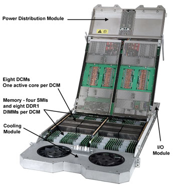
ASC Purple Chips and Modules:
- ASC Purple compute nodes are p5 575 nodes, which differ from standard p5
nodes in having only one active core in a dual-processor chip.
- With only one active cpu in a chip, the entire L2 and L3 cache is dedicated.
This design benefits scientific HPC applications by providing better
cpu-memory bandwidth.
- ASC Purple nodes are built from Dual-chip Modules (DCMs). Each node has a
total of eight DCMs. A photo showing these appears in the next section
below.
|
 |
Nodes
Node Characteristics:
- A node in terms of a POWER system, is defined as a single,
stand-alone, multi-processor machine, self-contained in a "box" which
is mounted in a frame. Nodes follow the "shared nothing"
model, which allows them to be "hot swappable".
- There is considerable variation in the types of POWER nodes IBM offers.
However, some common characteristics include:
- Uses one of the POWER family of processors
- SMP design - multiple processors (number of CPUs varies widely)
- Independent internal disk drives
- Network adapters, including adapter(s) for the internal switch network
- Memory resources, including memory cards and caches
- Power and cooling equipment
- Expansion slots for additional network and I/O devices
- Some types of nodes can be logically partitioned to look like multiple
nodes. For example, a 32-way POWER4 node could be made to look and
operate like 4 independent 8-way nodes.
- Typically, one copy of the operating system runs per node. However,
IBM does provide the means to run different operating systems on the
same node through partitioning.
Node Types:
- IBM packages its POWER nodes in a variety of ways, ranging from desktop
machines to supercomputers. Each variety is given an "official" IBM
model number/name. This is true for all POWER architectures.
- Within any given POWER architecture, models differ radically in how they
are configured: clock speed, physical size, number of CPUs, number of
I/O expansion slots, memory, price, etc.
- Most POWER nodes also have a "nickname" used in customer circles. The
nickname is often the "code name" born during the product's
"confidential" development cycle, which just happens to stick around
forever after.
- Some examples for nodes used by LC systems (past, present, future):
| LC Systems |
Node Model/Description |
Node Nickname |
| BLUE, SKY |
604e SMP 332 MHz, 4 CPUs |
Silver |
| WHITE, FROST |
POWER3 SMP 375 MHz High, 16 CPUs |
Nighthawk2, NH2 |
| UM, UV |
POWER4 pSeries p655, 1.5 GHz, 8 CPUs |
??? |
| BERG, NEWBERG |
POWER4 pSeries p690, 1.3 GHz, 32 CPUs |
Regatta |
| ASC PURPLE |
POWER5 p5 575, 1.9 GHz, 8 CPUs |
Squadron |
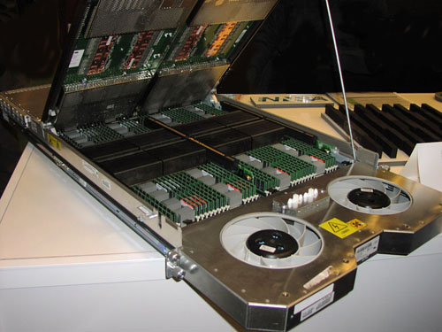
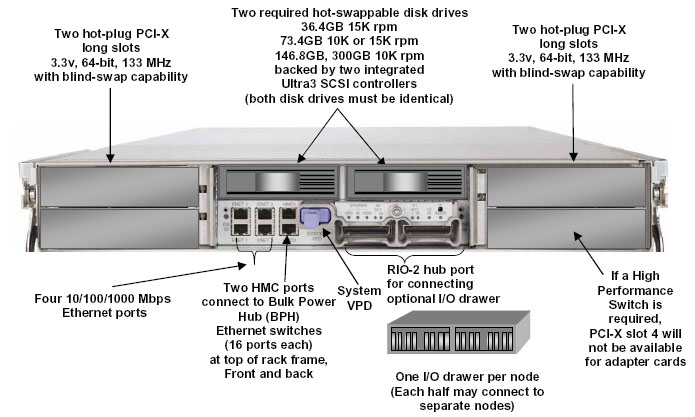
p5 575 Node:
- ASC Purple systems use p5 575 POWER5 nodes.
- "Innovative" 2U packaging - a novel design to minimize space requirements
and achieve "ultra dense" CPU distribution. Up to 192 CPUs per frame
(12 nodes * 16 CPUs/node).
- Eight Dual-chip Modules (DCMs) with associated memory
- Comprised of 4 "field swappable" component modules:
- I/O subsystem
- DC power converter/lid
- processor and memory planar
- cooling system
- I/O: standard configuration of two hot-swappable SCSI disk drives.
Expansion via an I/O drawer to 16 additional SCSI bays with a maximum
of 1.17 TB of disk storage.
- Adapters: standard configuration of four 10/100/1000 Mb/s ethernet
ports and two HMC ports. Expansion up to 4 internal PCI-X slots and
20 external PCI-X slots via the I/O drawer.
- Support for the High Performance Switch and InfiniBand
Frames
Frame Characteristics:

- Typical frames contain nodes, switch hardware, and frame hardware.
- Frame hardware includes:
- Redundant power supply units
- Air cooling hardware
- Control and diagnostic components
- Networking
- Frames are also used to house intermediate switch hardware
(covered later) and additional I/O, media and networking hardware.
- Frames can be used to "mix and match"
POWER components in a wide variety of ways.
- Frames vary in size and appearance, depending upon the type of
POWER system and what is required to support it.
- Several example POWER4 frame configurations (doors removed)
are shown below.
 |
|
- Power Supply
- 32-way POWER4 node
- 8-way POWER4 node
- Switch
- Intermediate switch
- I/O drawer
- Media Drawer
|
ASC Purple Frames:
- At LC, the early delivery ASC Purple machines are POWER4 nodes. The
final delivery systems contain POWER5 nodes.
- The frames that house ASC Purple compute nodes are shown below. They are
approximately 31"w x 80"h x 70"d (depth can vary).
- Also, as described previously, some frames are used to house
required intermediate switch hardware.
 |
 |
UM / UV |
PURPLE / UP |
Switch Network
Quick Intro:
- The switch network provides the internal, high
performance message passing fabric that connects every node to every
other node in a parallel POWER system.
- It has evolved along with the POWER architecture, and has been
called by various names along the way:
- High Performance Switch (HiPS)
- SP Switch
- SP Switch2
- Colony
- Federation
- HPS
- Currently, IBM is referring to its latest switch network as the
"High Performance Switch" or just "HPS", which interestingly enough,
is similar to what the very first switch network was called in the
days of the SP1.
- As would be expected, there are considerable differences between the
various switches, especially with regard to performance and
the types of nodes they are compatible with.
- For the interested, a history (an much, much more)
of the switch is presented in the IBM
Redbook called, "An Introduction to the New IBM eserver pSeries High
Performance Switch". Currently, this publication is available in PDF
format at:
www.redbooks.ibm.com/redbooks/pdfs/sg246978.pdf.
- The discussion here is limited (more or less) to a user's view of the
switch network and is highly simplified. In reality, the switch network
is very complicated. The same IBM redbook mentioned above covers in much
greater detail the "real" switch network, for the curious.
Topology:
- Bidirectional: Any-to-any internode connection allows all
processors to send messages simultaneously. Each point-to-point
connection between nodes is comprised of two channels
(full duplex) that can carry data in opposite directions
simultaneously.
- Multistage: On larger systems, additional
intermediate switches are required to scale the system upwards.
For example, with ASC Purple, there will be 3 levels of switches
required in order for every node to communicate with every other
node.

Switch Network Characteristics:
- Packet-switched network (versus circuit-switched). Messages are broken
into discrete packets and sent to their final destination, possibly
following different routes and out of sequence. All invisible to the
user.
- Support for multi-user environment - multiple jobs may run
simultaneously over the switch (one user does not monopolize switch)
- Path redundancy - multiple routings between any two nodes. Permits
routes to be generated even when there are faulty components in
the system.
- Built-in error detection
- Hardware redundancy for reliability - the switch board (discussed below)
actually uses twice as many hardware components as it minimally requires,
for RAS purposes.
- Architected for expansion to 1000s of ports. ASC Purple is the
first real system to prove this.
- Hardware components: in reality, the switch network is a very
sophisticated system with many complex components. From a user's
perspective however, there are only a few hardware components worth
mentioning:
- Switch drawers: house the switch boards and other support hardware.
Mounted in a frame.
- Switch boards: the heart of the switch network
- Switch Network Interface (SNI): an adapter that plugs into a node
- Cables: to connect nodes to switch boards and
switchboards to other switchboards
Switch Drawer:
- The switch drawer fits into a slot in a frame. For frames with
nodes, this is usually the bottom slot of a frame. For systems requiring
intermediate switches, there are frames dedicated to housing only switch
drawers.
- The switch drawer contains most of the components that comprise the
switch network, including but not limited to:
- Switchboard with switch chips
- Power supply
- Fans for cooling
- Switch port connector cards (riser cards)
Switch Board:
- The switch board is really the heart of the switch network.
The main features of the switch board are listed below.
- There are 8 logical Switch Chips, each of which is connected to 4 other
Switch Chips to form an internal 4x4 crossbar switch.
- A total of 32 ports controlled by Link Driver Chips on riser cards, are
used to connect to nodes and/or other switch boards.
- Depending upon how the Switch Board is used, it will be called a
Node Switch Board (NSB) or Intermediate Switch Board (ISB):
- NSB: 16 ports are configured for node connections. The other 16 ports
are configured for connections to switch boards in other frames.
- ISB: all ports are used to cascade to other switch boards.
- Practically speaking, the distinction between an NSB and ISB is
only one of topology. An ISB is just located higher up in the
network hierarchy.
- Switch-node connections are by copper cable. Switch-switch connections can
be either copper or optical fiber cable.
- Minimal hardware latency: approximately 59 nanoseconds to cross each Switch
Chip.
- Two simple configurations (96 node and 128 node systems)
using both NSB and ISB switch boards
are shown below. The number 4" refers to the number of ports connecting
each ISB to each NSB. Nodes are not shown, but each NSB may connect to 16
nodes.
|
 |
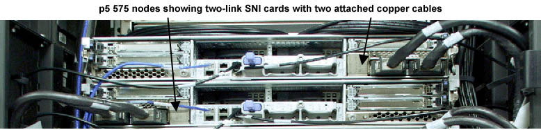
Switch Network Interface (SNI):
- The Switch Network Interface (SNI) is an adapter card that plugs into a
node's GX bus slot, allowing it to use the switch to communicate with other
nodes in the system. Every node that is connected to the switch must have
at least one switch adapter.
- There are different types of SNI cards. For example, p5 575 nodes use a
single, 2-link adapter card.
- One of the key features of the SNI is providing the ability for a process
to communicate via Direct Memory Access (DMA). Using DMA for communications
eliminates additional copies of data to system buffers; a process can
directly read/write to another process's memory.
- The node's adapter is directly cabled via a rather bulky copper
cable into a corresponding port on the switch board.
- There is much more to say about SNIs, but we'll leave that to the curious
to pursue in the previously mentioned (and other) IBM documentation.
Switch Communication Protocols:
- Applications can use one of two communications protocols, either
US or IP
- US - User Space Protocol. Preferred protocol due to performance.
Default at LC.
- IP - Internet Protocol. Slower but more "flexible". Used for
communications by jobs that span disjoint systems. Also used for
small systems that don't have a switch.
- Usage details are covered later in this tutorial.
Switch Application Performance:
- An application's communication performance over the switch is
dependent upon several factors:
- Node type
- Switch and switch adapter type
- Communications protocol used
- On-node vs. off-node proximity
- Application specific characteristics
- Network tuning parameters
- Competing network traffic
- Theoretical peak bi-directional performance: 4 GB/sec for POWER4/5
HPS (Federation) Switch
- Hardware latency: in practical terms, the switch hardware latency is
almost negligible when compared to the software latency involved in
sending data. Between any two nodes, hardware latency is in the range
of hundreds of nanoseconds (59 nanoseconds per switch chip crossed).
- Software latency comprises most of the delay in sending a message
between processes. To send MPI messages through the software stack over the switch incurs a latency of ~5 microseconds for the HPS switch.
- The table below demonstrates performance metrics for a 2 task,
MPI point-to-point (blocking) message passing program run on various
LC IBM systems.
- Note that these figures aren't even close to the theoretical peak figures.
Adding more MPI tasks would take full advantage of the switch/adapter
bandwidth and come closer to the theoretical peak.
Switch Type
Node Type |
Protocol |
Latency
(usec) |
Pt to Pt
Bandwidth
(MB/sec) |
Colony
POWER3 375 MHz |
IP |
105 |
77 |
| US |
20 |
390 |
HPS (Federation) Switch
POWER4 1.5 GHz |
IP |
32 |
318 |
| US |
6 |
3100 |
HPS (Federation) Switch
POWER5 1.9 GHz |
IP |
n/a |
n/a |
| US |
5 |
3100 |
GPFS Parallel File System
Overview:
- GPFS is IBM's General Parallel File System product.
- All of LC's parallel production POWER systems have at least one
GPFS file system.
- "Looks and feels" like any other UNIX file system from a user's
perspective.
- Architecture:
- Most nodes in a system are application/compute nodes
where programs actually run. A subset of the system's nodes are
dedicated to serve as storage nodes for conducting
I/O activities between the compute nodes and physical disk. Storage
nodes are the interface to disk resources.
- For performance reasons, data transfer between the application nodes
and storage nodes typically occurs over the internal switch network.

- Individual files are stored as a series of "blocks" that are striped
across the disks of different storage nodes. This permits concurrent
access by a multi-task application when tasks read/write to different
segments of a common file.
- Internally, GPFS's file striping is set to a specific block
size that is configurable. At LC, the most efficient use of GPFS is
with large files. The use of many small files in a GPFS file system
is not advised if performance is important.
- IBM's implementation of MPI-IO routines depends upon an underlying GPFS
system to accomplish parallel I/O within MPI programs.
- GPFS Parallelism:
- Simultaneous reads/writes to non-overlapping regions of the same file
by multiple tasks
- Concurrent reads and writes to different files by multiple tasks
- I/O will be serial if tasks attempt to use the same stripe of a file
simultaneously.
- Additional information: Search
ibm.com for "GPFS".
LC Configuration Details:
- Naming scheme: /p/gscratch#/username where:
- # = one digit number on the SCF; one character alpha on the OCF
(ex: gscratch1, gscratcha).
- username = your user name on that machine. Established automatically.
- Symbolic links allow for standardized naming in scripts, etc.:
/p/glocal1, /p/glocal2 link to local GPFS file systems.
- Configurations:
- Sizes of GPFS file systems vary between systems. And they change.
- A machine may have more than one GPFS file system.
- Sizes change from time to time. du -k will tell you
what the current configuration.
- GPFS file systems are not global; they are local to a specific system.
- At LC, GPFS file systems are configured optimally for use with large
data files.
- Temporary location:
- No backup
- Purge policies are in effect, since a full file system reduces
performance.
- Not reliable for long term storage
General Configuration:
- All of LCs production, parallel POWER systems follow the general
configuration schematic shown below.
- Most nodes are designated as compute nodes
- Some nodes are dedicated as file servers to the GPFS parallel file
system(s)
- A few nodes serve exclusively as login machines
- All nodes are internally connected by a high speed switch
- Access to HPSS storage and external systems is over a GigE network
SCF POWER Systems
ASC PURPLE:
| Purpose: |
ASC Capability Resource |
| Nodes: |
1532 |
| CPUs/Node: |
8 |
| CPU Type: |
POWER5 p5 575 @1.9 GHz |
| Peak Performance: |
93 TFLOPS |
| Memory/Node: |
32 GB |
| Memory Total: |
49 TB |
| Cache: |
32 KB L1 data; 64 KB L1 instruction; 1.9 MB L2; 36 MB L3 |
| Interconnect: |
IBM High Performance Switch (HPS) |
| Parallel File System: |
GPFS |
| OS: |
AIX |
| Notes: |
Photo below
Login nodes differ from compute nodes:
- Two 32-way POWER5 machines partitioned to look like four 16-way machines
- 64 GB memory
Additional info:
asc.llnl.gov/computing_resources/purple
|
UM and UV:
| Purpose: |
ASC Capacity Resources
Two nearly identical resources. Information below is for each system. |
| Nodes: |
128 |
| CPUs/Node: |
8 |
| CPU Type: |
POWER4 p655 @1.5 GHz |
| Peak Performance: |
6.1 TFLOPS |
| Memory/Node: |
16 GB |
| Memory Total: |
2 TB |
| Cache: |
32 KB L1 data; 64 KB L1 instruction; 1.44 MB L2; 32 MB L3 |
| Interconnect: |
IBM High Performance Switch (HPS) |
| Parallel File System: |
GPFS |
| OS: |
AIX |
| Notes: |
Part of ASC Purple "early delivery".
Photo below |
TEMPEST:
| Purpose: |
ASC Single-node or serial computing |
| Nodes: |
12 |
| CPUs/Node: |
9 nodes with 4 CPUs/node
3 nodes with 16 CPUs/node |
| CPU Type: |
4-way nodes: POWER5 p5 550 @1.65 GHz
16-way nodes: POWER5 p5 570 @1.65 GHz |
| Peak Performance: |
554 GFLOPS |
| Memory/Node: |
4-way nodes: 32 GB
16-way nodes: 64 GB |
| Memory Total: |
480 GB |
| Cache: |
32 KB L1 data; 64 KB L1 instruction; 1.9 MB L2; 36 MB L3 |
| Interconnect: |
None |
| Parallel File System: |
None |
| OS: |
AIX |
| Notes: |
Only 4-way or 16-way parallel jobs (depending upon the node) because there
is no switch interconnect (single node parallelism).
See /usr/local/docs/tempest.basics for more information. |
OCF POWER Systems
UP:
| Purpose: |
ASC Capacity Resource |
| Nodes: |
108 |
| CPUs/Node: |
8 |
| CPU Type: |
POWER5 p5 575 @1.9 GHz |
| Peak Performance: |
6.6 TFLOPS |
| Memory/Node: |
32 GB |
| Memory Total: |
3 TB |
| Cache: |
32 KB L1 data; 64 KB L1 instruction; 1.9 MB L2; 36 MB L3 |
| Interconnect: |
IBM High Performance Switch (HPS) |
| Parallel File System: |
GPFS |
| OS: |
AIX |
| Notes: |
UP stands for "Unclassified Purple" |
BERG, NEWBERG:
| Purpose: |
Non-production, testing, prototyping |
| Nodes: |
2 |
| CPUs/Node: |
32 |
| CPU Type: |
POWER5 p4 690 @1.3 GHz |
| Peak Performance: |
166 GFLOPS |
| Memory/Node: |
32 GB |
| Memory Total: |
64 GB |
| Cache: |
32 KB L1 data; 64 KB L1 instruction; 1.44 MB L2; 32 MB L3 |
| Interconnect: |
IBM High Performance Switch (HPS) |
| Parallel File System: |
None |
| OS: |
AIX |
| Notes: |
BERG: Single 32-processor machine configured into 3 logical nodes
NEWBERG: Single 32-processor machine configured into 4 logical nodes
Photo
|
|
Software and Development Environment
|
The software and development environment for the IBM SPs at LC
is similar to what is described in the Introduction to LC Resources tutorial. Items specific
to the IBM SPs are discussed below.
AIX Operating System:
- AIX is IBM's proprietary version of UNIX.
- In the past, AIX was the only choice of operating system for
POWER machines. Now, Linux can be used on POWER systems also.
- As mentioned earlier, AIX is "Linux friendly", which means:
- That many solutions developed under Linux will run under AIX 5L by
simply recompiling the source code.
- IBM provides the "AIX Toolbox for Linux
Applications" which is a collection of Open Source and GNU software
commonly found with Linux distributions.
- LC currently uses only AIX for all of its IBM systems. Every SMP node
runs under a single copy of the AIX operating system, which is
threaded for all CPUs.
- Beginning with POWER5 and AIX 5.3, simultaneous multithreading is supported.
Micro-partitioning (multiple copies of an OS on a single processor)
is also supported.
- AIX product information and complete documentation are
available from IBM on the web at www-03.ibm.com/servers/aix
Parallel Environment:
- IBM's Parallel Environment is a collection of software tools and
libraries designed for developing, executing, debugging and profiling
parallel C, C++ and Fortran applications on POWER systems running AIX.
- The Parallel Environment consists of:
- Parallel Operating Environment (POE) software for submitting and
managing jobs
- IBM's MPI library
- A parallel debugger (pdbx) for debugging parallel programs
- Parallel utilities for simplified file manipulation
- PE Benchmarker performance analysis toolset
- Parallel Environment documentation can be found in
IBM's Parallel Environment manuals.
Parallel Environment topics are also discussed in the
POE section below.
Compilers:
- IBM - C/C++ and Fortran compilers. Covered
later.
- gcc, g++, g77 - GNU C, C++ and Fortran compilers
- Guide - KAI OpenMP C, C++ and Fortran compilers. Available but no
longer officially supported by LC.
Math Libraries Specific to IBM SPs:
- ESSL - IBM's Engineering Scientific Subroutine Library.
- PESSL - IBM's Parallel Engineering Scientific Subroutine Library.
A subset of ESSL that has been parallelized. Documentation is located with
ESSL documentation mentioned above.
- MASS - Math Acceleration Subsystem. High performance versions of
most math intrinsic functions. Scalar versions and vector versions. See
/usr/local/lpp/mass or search IBM's web pages for more information.
Batch Systems:
- LCRM - LC's legacy batch system. Covered in the
LCRM Tutorial.
Currently being migrated to Moab.
- Moab - New Tri-lab batch system. Covered in the
Moab Tutorial.
- SLURM - LC's native resource manager system, which resides
"under" LCRM/Moab. Stands for
"Simple Linux Utility for Resource Management".
More information available at: computing.llnl.gov/linux/slurm.
User Filesystems:
- As usual - home directories, /nfs/tmp, /var/tmp, /tmp,
/usr/gapps, archival storage. For more information see the
Introduction to LC Resources tutorial.
- General Parallel File System (GPFS) - IBM's parallel filesystem
available on LC's parallel production IBM systems. GPFS is discussed in the
Parallel File Systems section of the Introduction
to Livermore Computing Resources tutorial.
Software Tools:
- In addition to compilers, LC's Development Environment Group (DEG)
supports a wide variety of software tools including:
- Debuggers
- Memory tools
- Profilers
- Tracing and instrumentation tools
- Correctness tools
- Performance analysis tools
- Various utilities
- Most of these tools are simply listed below.
For detailed information see
computing.llnl.gov/code/content/software_tools.php.
- Debugging/Memory Tools:
- TotalView
- dbx
- pdbx
- gdb
- decor
- Tracing, Profiling, Performance Analysis and Other"Tools:
- prof
- gprof
- PE Benchmarker
- IBM HPC Toolkit
- TAU
- VampirGuideView (VGV)
- Paraver
- mpiP
- Xprofiler
- mpi_trace
- PAPI
- PMAPI
- Jumpshot
- Dimemas
- Assure
- Umpire
- DPCL
Video and Graphics Services:
- LC's Information Management and Graphics Group (IMGG) provides a range of
visualization hardware, software and services including:
- Parallel visualization clusters
- PowerWalls
- Video production
- Consulting for scientific visualization issues
- Installation and support of visualization and graphics software
- Support for LLNL Access Grid nodes
- Contacts and more information:
|
Parallel Operating Environment (POE) Overview
|
Most of what you'll do on any parallel IBM AIX POWER system will be under IBM's Parallel Operating Environment (POE) software. This section provides a quick
overview. Other sections provide the details for actually using POE.
PE vs POE:
- IBM's Parallel Environment (PE) software product encompasses a
collection of software tools designed to provide a complete
environment for developing, executing, debugging and profiling
parallel C, C++ and Fortran programs.
- As previously mentioned, PE's primary components include:
- Parallel compiler scripts
- Facilities to manage your parallel execution environment (environment
variables and command line flags)
- Message Passing Interface (MPI) library
- Low-level API (LAPI) communication library
- Parallel file management utilities
- Authentication utilities
- pdbx parallel debugger
- PE Benchmarker performance analysis toolset
- Technically, the Parallel Operating Environment (POE) is a subset
of PE that actually contains the majority of the PE product.
- However, to the user this distinction is not really necessary
and probably serves more to confuse than enlighten. Consequently,
this tutorial will consider PE and POE synonymous.
Types of Parallelism Supported:
- POE is primarily designed for process level (MPI) parallelism, but fully
supports threaded and hybrid (MPI + threads) parallel programs also.
- Process level MPI parallelism is directly managed by POE from
compilation through execution.
- Thread level parallelism is "handed off" to the compiler, threads
library and OS.
- For hybrid programs, POE manages the MPI tasks, and
lets the compiler, threads library and OS manage the threads.
- POE fully supports Single Process Multiple Data (SPMD) and
Mutltiple Process Multiple Data (MPMD) models for parallel programming.
- For more information about parallel programming, MPI, OpenMP and
POSIX threads, see the tutorials listed on the
LC Training web page.
Interactive and Batch:
- POE can be used both interactively and within a batch scheduler
system to compile, load and run parallel jobs.
- There are many similarities between interactive and batch POE usage.
There are also important differences. These will
be pointed out later as appropriate.
Typical Usage Progression:
- The typical progression of steps for POE usage is outlined below,
and discussed in more detail in following sections.
- Understand your system's configuration (always changing?)
- Establish POE authorization on all nodes that you will use (one-time
event for some. Not even required at LC.)
- Compile and link the program using one of the POE parallel
compiler scripts. Best to do this on the actual platform you want
to run on.
- Set up your execution environment by setting the necessary POE
environment variables. Of course, depending upon your application,
and whether you are running interactively or batch, you may need
to do a lot more than this. But we're only talking about POE here...
- Invoke the executable - with or w/o POE options
A Few Miscellaneous Words About POE:
- POE is unique to the IBM AIX environment. It runs only on the IBM POWER
platforms under AIX.
- Much of what POE does is designed to be transparent to the user.
Some of these tasks include:
- Linking to the necessary parallel libraries during compilation (via
parallel compiler scripts)
- Finding and acquiring requested machine resources for your parallel job
- Loading and starting parallel tasks
- Handling all stdin, stderr and stdout for each parallel task
- Signal handling for parallel jobs
- Providing parallel communications support
- Managing the use of processor and network resources
- Retrieving system and job status information
- Error detection and reporting
- Providing support for run-time profiling and analysis tools
- POE can also be used to run serial jobs and shell commands concurrently
across a network of machines. For example, issuing the command
poe hostname
will cause each machine in your partition
to tell you its name. Run just about any other shell command or
serial job under poe and it will work the same way.
- POE limts (number of tasks, message sizes, etc.) can be found in the
MPI Programming Guide Parallel Environment
manual (see the chapter on Limits).
Some POE Terminology:
Before learning how to use POE, understanding some basic definitions may
be useful. Note that some of these terms are common to parallel programming
in general while others are unique or tailored to POE.
- Node
- Within POE, a node usually refers to single machine, running
its own copy of the AIX operating system. A node has a unique network
name/address. All current model IBM nodes are SMPs (next).
- SMP
- Symmetric Multi-Processor. A computer (single machine/node) with
multiple CPUs that share a common memory. Different types of SMP nodes may
vary in the number of CPUs they possess and the manner in which the
shared memory is accessed.
- Process / Task
- Under POE, an executable (a.out) that may be scheduled to run
by AIX on any available physical processor as a UNIX process is
considered a task. Task and process are synonymous. For MPI applications,
each MPI process is referred to as a "task" with a unique identifier
starting at zero up to the number of processes minus one.
- Job
- A job refers to the entire parallel application and typically consists
of multiple processes/tasks.
- Interprocess
- Between different processes/tasks. For example, interprocess
communications can refer to the exchange of data between different
MPI tasks executing on different physical processors. The processors
can be on the same node (SMP) or on different nodes, but with POE, are
always part of the same job.
- Pool
- A pool is an arbitrary collection of nodes assigned by system managers.
Pools are typically used to
separate nodes into disjoint groups, each of which is used for specific
purposes. For example, on a given system, some nodes may be designated
as "login" nodes, while others are reserved for "batch" or "testing"
use only.
- Partition
- The group of nodes used to run a parallel job is
called a partition. Across a system, there is one discreet
partition for each user's job. Typically, the nodes in a
partition are used exclusively by a single user for the
duration of a job. (Technically though, POE allows multiple users to
share a partition, but in practice, this is not common, for obvious
reasons.) After a job completes, the nodes may be
allocated for other users' partitions.
- Partition Manager
- The Partition Manager, also known as the poe daemon,
is a process that is automatically started for each parallel job.
The Partition Manager is responsible for overseeing the parallel
execution of the job by communicating with daemon processes on each node
in the partition and with the system scheduler. It operates transparently
to the user and terminates after the job completes.
- Home Node / Remote Node
- The home node is the node where the parallel job is initiated
and where the Partition Manager process lives.
The home node may or may not be considered part of your partition
depending upon how the system is configured, interactive vs. batch, etc.
A Remote Node is any other node in your partition.
|
|
Compilers and Compiler Scripts:
- In IBM's Parallel Environment, there are a number of compiler invocation
commands, depending upon what you want to do. However, underlying all
of these commands are the same AIX C/C++ and Fortran compilers.
- The POE parallel compiler commands are actually scripts that
automatically link to the necessary Parallel Environment libraries,
include files, etc. and then call the appropriate native AIX compiler.
- For the most part, the native IBM compilers and their parallel
compiler scripts support a common command line syntax.
- See the References and More Information section
for links to IBM compiler documentation. Versions change frequently and
downloading the relevant documentation from IBM is probably the best
source of information for the version of compiler you are using.
Compiler Syntax:
[compiler] [options] [source_files] |
For example:
mpxlf -g -O3 -qlistopt -o myprog mprog.f
Common Compiler Invocation Commands:
- Note that all of the IBM compiler invocation commands are not shown.
Other compiler commands are available to select IBM compiler extensions
and features. Consult the appropriate IBM compiler man page and compiler
manuals for details. Man pages are linked below for convenience.
- Also note, that since POE version 4, all commands actually use the
_r (thread-safe) version of the command. In other words,
even though you compile with xlc, you will really get the
xlc_r thread-safe version of the compiler.
| IBM Compiler Invocation Commands |
| Serial |
xlc
cc |
ANSI C compiler
Extended C compiler (not strict ANSI) |
| xlC |
C++ compiler |
xlf
f77 |
Extended Fortran; Fortran 77 compatible
xlf alias |
xlf90
f90 |
Full Fortran 90 with IBM extensions
xlf90 alias |
xlf95
f95 |
Full Fortran 95 with IBM extensions
xlf95 alias |
Threads
(OpenMP,
Pthreads,
IBM threads) |
xlc_r / cc_r |
xlc / cc for use with threaded programs |
| xlC_r |
xlC for use with threaded programs |
| xlf_r |
xlf for use with threaded programs |
| xlf90_r |
xlf90 for use with threaded programs |
| xlf95_r |
xlf95 for use with threaded programs |
| MPI |
mpxlc / mpcc |
Parallel xlc / cc compiler scripts |
| mpCC |
Parallel xlC compiler script |
| mpxlf |
Parallel xlf compiler script |
| mpxlf90 |
Parallel xlf90 compiler script |
| mpxlf95 |
Parallel xlf95 compiler script |
MPI with
Threads
(OpenMP,
Pthreads,
IBM threads) |
mpxlc_r / mpcc_r |
Parallel xlc / cc compiler scripts for hybrid MPI/threads programs |
| mpCC_r |
Parallel xlC compiler script for hybrid MPI/threads programs |
| mpxlf_r |
Parallel xlf compiler script for hybrid MPI/threads programs |
| mpxlf90_r |
Parallel xlf90 compiler script for hybrid MPI/threads programs |
| mpxlf95_r |
Parallel xlf95 compiler script for hybrid MPI/threads programs |
Compiler Options:
- IBM compilers include many options - too
numerous to be covered here. For a full discussion, consult the IBM
compiler documentation. An abbreviated summary of some common/useful
options are listed in the table below.
| Option |
Description |
C/C++ |
Fortran |
-blpdata |
Enable executable for large pages. Linker option. See
Large Pages discussion. |
 |
 |
-bbigtoc |
Required if the image's table of contents (TOC) is greater than 64KB. |
|
|
-c |
Compile only, producing a ".o" file. Does not link object
files. |
|
|
-g |
Produce information required by debuggers and some
profiler tools |
|
|
-I |
Names directories for additional include files. |
|
|
-L |
Specifies pathname where additional libraries reside
directories will be searched in the order of their occurrence on
the command line. |
|
|
-l |
Names additional libraries to be searched. |
|
|
-O -O2 -O3 -O4 -O5 |
Various levels of optimization. See discussion below. |
|
|
-o |
Specifies the name of the executable (a.out by default) |
|
|
-p -pg |
Generate profiling support code. -p is required for use with
the prof utility and -pg is required for use with the
gprof utility. |
|
|
-q32, -q64 |
Specifies generation of 32-bit or 64-bit objects. See discussion
below. |
|
|
-qhot |
Determines whether or not to perform high-order
transformations on loops and array language during
optimization, and whether or not to pad array dimensions
and data objects to avoid cache misses. |
|
|
-qipa |
Specifies interprocedural analysis optimizations |
|
|
-qarch=arch
-qtune=arch |
Permits maximum optimization for the processor
architecture being used. Can improve performance at the
expense of portability. It's probably best to use auto
and let the compiler optimize for the platform where you actually compile.
See the man page for other options. |
|
|
-qautodbl=setting |
Automatic conversion of single precision to double
precision, or double precision to extended precision. See the man page
for correct setting options. |
|
|
-qreport |
Displays information about loop transformations if -qhot or
-qsmp are used. |
|
|
-qsmp=omp |
Specifies OpenMP compilation |
|
|
-qstrict |
Turns off aggressive optimizations which have the potential to alter the
semantics of a user's program. |
|
|
-qlist
-qlistopt
-qsource
-qxref |
Compiler listing/reporting options. -qlistopt may be of use
if you want to know the setting of ALL options. |
|
|
-qwarn64 |
Aids in porting code from a 32-bit environment to a 64-bit environment
by detecting the truncation of an 8 byte integer to 4 bytes. Statements
which may cause problems will be identified through informational messages.
|
|
|
-v -V |
Display verbose information about the compilation |
|
|
-w |
Suppress informational, language-level, and warning messages. |
|
|
-bmaxdata:bytes |
Historical. This is actually a loader (ld) flag required for
use on 32-bit objects that exceed the default data segment
size, which is only 256 MB, regardless of the machine's
actual memory. At LC, this option would not normally be used because all
of its IBM systems are now 64-bit since the retirement of the ASC Blue
systems. Codes that link to old libraries compiled in 32-bit mode
may still need this option, however. |
|
|
32-bit versus 64-bit:
- LC's POWER4 and POWER5 machines default to 64-bit compilations.
- In the past, LC operated the 32-bit ASC Blue machines.
- Because 32-bit and 64-bit executables are incompatible, users needed to
be aware of the compilation mode for all files in their application. An
executable has to be entirely 32-bit or entirely 64-bit. An example of
when this might be a problem would be trying to link old 32-bit
executables/libraries into your 64-bit application.
- Recommendation: explicitly specify your compilations with either -q32 or
-q64 to avoid any problems encountered by accepting the defaults.
Optimization:
- Default is no optimization
- Without the correct -O option specified, the defaults for
-qarch and -qtune are not optimal!
Only -O4 and -O5 automatically select the best
architecture related optimizations.
- -O4 and -O5 can perform optimizations specific to L1
and L2 caches on a given platform. Use the -qlistopt flag
with either of these and then look at the listing file for this
information.
- Any level of optimization above -O2 can be aggressive and change
the semantics of your program, possibly reduce performance or cause
wrong results. You can use -qstrict flag with the
higher levels of optimization to restrict semantic changing optimizations.
- The compiler uses a default amount of memory to perform optimizations.
If it thinks it needs more memory to do a better job, you may get a
warning message about setting MAXMEM to a higher value. If you specify
-qmaxmem=-1 the compiler is free to use as much memory as it needs
for its optimization efforts.
- Optimizations may cause the compiler to relax conformance to the IEEE
Floating-Point Standard.
Miscellaneous:
- Conformance to IEEE Standard Floating-Point Arithmetic: the IBM C/C++
and Fortran compilers "mostly" follow the standard, however, the
exceptions and discussions are too involved to cover here.
- The IBM documentation states that the
C/C++ and Fortran compilers support OpenMP version 2.5.
- All of the IBM compiler commands have default options, which can
be configured by a site's system adminstrators. It may be useful to
review the files /etc/*cfg* to learn exactly what the
defaults are for the system you're using.
- Static Linking and POE: POE executables that use MPI are
dynamically linked with the appropriate communications library at
run time. Beginning with POE version 4, there is no support for
building statically bound executables.
- The IBM C/C++ compilers automatically support POSIX threads - no
special compile flag(s) are needed. Additionally, the IBM Fortran
compiler provides an API and support for pthreads even though there
is no POSIX API standard for Fortran.
See the IBM Documentation - Really!
Implementations:
- On LC's POWER4 and POWER5 systems, the only MPI library available is IBM's
thread-safe MPI. It includes MPI-1 and most of MPI-2 (excludes dynamic
processes).
- MPI is automatically linked into your build when you use any of the
compiler commands below. Recall as discussed earlier, the thread-safe
version of the compiler (_r version) is automatically used at LC even
if you call the non _r version.
| IBM MPI Compiler Invocation Commands |
| MPI |
mpxlc / mpcc |
Parallel xlc / cc compiler scripts |
| mpCC |
Parallel xlC compiler script |
| mpxlf |
Parallel xlf compiler script |
| mpxlf90 |
Parallel xlf90 compiler script |
| mpxlf95 |
Parallel xlf95 compiler script |
MPI with
Threads
(OpenMP,
Pthreads,
IBM threads) |
mpxlc_r / mpcc_r |
Parallel xlc / cc compiler scripts for hybrid MPI/threads programs |
| mpCC_r |
Parallel xlC compiler script for hybrid MPI/threads programs |
| mpxlf_r |
Parallel xlf compiler script for hybrid MPI/threads programs |
| mpxlf90_r |
Parallel xlf90 compiler script for hybrid MPI/threads programs |
| mpxlf95_r |
Parallel xlf95 compiler script for hybrid MPI/threads programs |
Notes:
- All MPI compiler commands are actually "scripts" that automatically link
in the necessary MPI libraries, include files, etc. and then call the
appropriate native AIX compiler.
- Documentation for the IBM implementation is available
from IBM.
- LC's MPI tutorial describes
how to create MPI programs.
|
Running on LC's POWER Systems
|
Large Pages
Large Page Overview:
- IBM AIX page size has typically been 4KB. Beginning with POWER4 and AIX 5L
version 5.1, 16MB large page support was implemented.
- The primary purpose of large pages is to provide performance improvements
for memory intensive HPC applications. The performance improvement
results from:
- Reducing translation look-aside buffer (TLB) misses through mapping
more virtual memory into the TLB. TLB memory coverage for large pages is
16 GB vs. 4 MB for small pages.
- Improved memory prefetching by eliminating the need to restart prefetch
operations on 4KB boundaries. Large pages hold 131,072 cache lines vs.
32 cache lines for 4KB pages.
- AIX treats large pages as pinned memory - an application's data remains
in physical memory until the application completes. AIX does not provide
paging support for large pages.
- According to IBM, memory bandwidth can be increased up to 3x for some
applications when using large pages. In practice this may translate to
an overall application speedup of 5-20%.
- However, some applications may demonstrate a marked decrease in
performance with large pages:
- Short running applications (measured in minutes)
- Applications that perform fork() and exec() operations
- Shell scripts
- Compilers
- Graphics tools
- GUIs for other tools (such as TotalView)
- If large pages are exhausted, enabled applications silently fail over to
use small pages, with possible ramifications to performance. However,
the converse is not true: applications that use only small pages cannot
access large-page memory.
- Large page configuration is controlled by system managers. Using this
configuration is entirely up to the user. It is not automatic.
- More information: AIX Support For
Large Pages whitepaper.
Large Pages and Purple:
- Purple systems are configured to allocate the maximum AIX permitted
amount (85%) of a machine's memory for large pages. This means that there
is a relatively small amount of memory available for regular 4KB pages.
- IMPORTANT: Because LC has allocated most of memory for large pages,
applications which aren't enabled for large pages will default to using
the limited 4KB page pool. It is quite likely in such cases that excessive
paging will occur and the job will have to be terminated to prevent
it from hanging or crashing the system.
How to Enable Large Pages:
- As mentioned, even though a system has large pages configured, making
use of them is up to the user.
- Use any of three ways to enable an application for large page use:
- At build time: link with the -blpdata flag.
Recommended.
- After build: use the ldedit -blpdata executable
command on your executable. Recommended.
- At runtime: set the LDR_CNTRL=LARGE_PAGE_DATA=Y environment
variable. For example:
setenv LDR_CNTRL=LARGE_PAGE_DATA=Y
Note that if you foget to unset this environment variable after your
application runs, this method will affect all other tasks in your
login session. Routine, non-application tasks will probably be
very slow, and it is therefore NOT recommended for interactive jobs
where you are using other tools/utilities.
When NOT to Use Large Pages:
- In most cases, large pages should not be used for non-application tasks
such as editing, compiling, running scripts, debugging, using
GUIs or running non-application tools. Using large pages for these tasks
will cause them to perform poorly in most cases.
- Using the LDR_CNTRL=LARGE_PAGE_DATA=Y environment variable will cause
all tasks to use large pages, not just your executable. For this reason,
it is not recommended.
- Of special note: do not run TotalView under large pages. Discussed
later in the Debugging section of this
tutorial.
- To change a large page executable to not use large pages, use the
command lededit -bnolpdata executable
Miscellaneous Large Page Info:
- To see if the large page bit is set on an executable, use the command
shown below. Note that the example executable's name is "bandwidth"
and that the output will contain LPDATA if the bit is set.
% dump -Xany -ov bandwidth | grep "Flags"
Flags=( EXEC DYNLOAD LPDATA DEP_SYSTEM )
|
- On AIX 5.3 and later, "ps -Z" will show 16M in the DPGSZ column (data
page size) for jobs using large pages. The SPGSZ (stack) and TPGSZ
(text) columns will remain at 4K regardless. For example:
% ps -Z
   PID    TTY  TIME DPGSZ SPGSZ TPGSZ CMD
135182 pts/68  0:00    4K    4K    4K my_small_page_job
177982 pts/68  0:00   16M    4K    4K my_large_page_job
|
- The sysconf(_SC_LARGE_PAGE_SIZE) function call will return the large
page size on systems that have large pages.
- The vmgetinfo() function returns information about large page pools
size and other large page related information.
|
Running on LC's POWER Systems
|
SLURM
LC's Batch Schedulers:
- The native (low level) scheduling software provided by IBM for parallel
POWER systems is LoadLeveler. At LC, LoadLeveler has been replaced by
SLURM.
- SLURM resource manager:
- SLURM = Simple Linux Utility for Resource Management
- Developed by LC; open source
- Also used on all of LC's Linux clusters
- SLURM manages a single cluster - it does not know about other
clusters - hence "low level".
- LC's system-wide batch schedulers (high-level; workload managers)
are LCRM and Moab:
- LCRM/Moab "talk" to the low-level SLURM resource manager on each
system.
- Tie multiple clusters into an enterprise-wide system
- LCRM and Moab are discussed in detail in the
LCRM tutorial and
Moab tutorial.
SLURM Architecture:
- SLURM is implemented with two daemons:
- slurmctld - central management daemon.
Monitors all other SLURM daemons and resources, accepts work
(jobs), and allocates resources to those jobs. Given the
critical functionality of slurmctld, there may be a backup
daemon to assume these functions in the event that the
primary daemon fails.
- slurmd - compute node daemon. Monitors all
tasks running on the compute node, accepts work (tasks),
launches tasks, and kills running tasks upon request.

- SLURM significantly alters the way POE behaves, especially in batch.
- There are differences between the SLURM implementation on POWER systems
and the SLURM implementation on LC's Linux systems.
SLURM Commands:
- SLURM provides six user-level commands. Note that the IBM implementation
does not support all six commands. Commands are linked to their
corresponding man page.
| SLURM Command |
Description |
Supported on IBMs? |
| scancel |
Cancel or signal a job |
INTERACTIVE ONLY |
| scontrol |
Administration tool; configuration |
YES |
| sinfo |
Reports general system information |
YES |
| smap |
Displays an asci-graphical version of squeue |
YES |
| squeue |
Reports job information |
YES |
| srun |
Submits/initiates a job |
NO |
SLURM Environment Variables:
- The srun man page describes a
number of SLURM environment variables. However, under AIX, only a few
of these are supported (described below).
| SLURM Environment Variable |
Description |
| SLURM_JOBID |
Use with "echo" to display the jobid. |
| SLURM_NETWORK |
Specifies switch and adapter settings such as communication protocol, RDMA
and number of adapter ports. Replaces the use
of the POE MP_EUILIB and MP_EUIDEVICE environment
variables. In most cases, users should not modify the default settings, but
if needed, they can. For example to run with IP protocol over a single
switch adapter port:
setenv SLURM_NETWORK ip,sn_single
The default setting is to use User Space protocol over both switch adapter
ports and to permit RDMA.
setenv SLURM_NETWORK us,bulk_xfer,sn_all |
| SLURM_NNODES |
Specify the number of nodes to use. Currently not working
on IBM systems. |
| SLURM_NPROCS |
Specify the number of processes to run. The default is one process
per node. |
Additional Information:
|
Running on LC's POWER Systems
|
Understanding Your System Configuration
First Things First:
- Before building and running your parallel application, it is important
to know a few details regarding the system you intend to use.
This is especially important if you use multiple systems, as they will
be configured differently.
- Also, things at LC are in a continual state of flux. Machines change,
software changes, etc.
- Several information sources and simple configuration commands
are available for understanding LC's IBM systems.
System Configuration/Status Information:
- LC's Home Page: computing.llnl.gov
- Important Notices and News - timely information for every system
- OCF Machine Status (LLNL internal) - shows if the machine is up or
down and then links to the following information for each machine:
- Message of the Day
- Announcements
- Load Information
- Machine Configuration (and other) information
- Job Limits
- Purge Policy
- Computing Resources - detailed machine configuration information
for all machines.
- When you login, be sure to check the login banner & news items
- Machine status email lists.
- Each machine has a status list which provides the most timely
status information and plans for upcoming system maintenance or
changes. For example:
uv-status@llnl.gov
um-status@llnl.gov
up-status@llnl.gov
...
- LC support initially adds people to the list, but just in case you
find you aren't on a particular list (or want to get off), just use
the usual majordomo commands in an email sent to
Majordomo@lists.llnl.gov.
LC Configuration Commands:
-
ju: Displays a summary of node availability
and usage within each pool. Sample output, partially truncated, shown below.
uv006% ju
Partition     total down used avail  cap Jobs
systest           4    0    0     4   0%
pdebug            2    0    1     1  50% degrt-2
pbatch 99 0 92 7 93% halbac-8, fdy-8, fkdd-8, kuba-16, dael-6 |
-
spjstat: Displays a summary of pool information followed
by a listing of all running jobs, one job per line.
Sample output, partially truncated, shown below.
up041% spjstat
Scheduling pool data:
--------------------------------------------------------
Pool      Memory    Cpus Nodes Usable Free  Other traits
--------------------------------------------------------
pbatch   31616Mb       8    99     99    8
pdebug   31616Mb       8     2      1    1
systest  31616Mb       8     4      4    4

Running job data:

-------------------------------------------------------
Job ID         User Name    Nodes    Pool     Status
-------------------------------------------------------
11412          dael            6     pbatch     Running
28420          hlbac           8     pbatch     Running
28040          rtyg            6     pbatch     Running
30243 kubii 16 pbatch Running |
-
sinfo: SLURM systems only.
Displays a summary of the node/pool configuration. Sample output below.
up041% sinfo
PARTITION AVAIL  TIMELIMIT NODES  STATE NODELIST
pbatch*      up   infinite    91  alloc up[001-016,021-036,042-082,089-106]
systest      up    2:00:00     4   idle up[085-088]
pdebug       up    2:00:00     1   idle up037
pdebug       up    2:00:00     1   comp up040
pbatch* up infinite 8 idle up[017-020,083-084,107-108] |
IBM Configuration Commands:
- Several standard IBM AIX and Parallel Environment commands that may prove
useful are shown below. See the man pages for usage details.
- lsdev: This command lists all of the available
physical devices (disk, memory, adapters, etc.)
on a single machine. Probably its most useful purpose
after providing a list, is that it tells you the names of devices
you can use with the lsattr command for detailed information.
Sample output
- lsattr: Allows you to obtain detailed information for
a specific device on a single machine. The catch is you need to
know the device name, and
for that, the previously mentioned lsdev command is used.
Sample output
- lslpp -al | grep poe: The lslpp command is used
to check on installed software. If you grep the output for poe
it will show you which version of POE is installed on that machine.
- Note that the serial lsattr, lsdev, and lslpp commands
can be used in parallel simply by calling them via poe. For example,
if the following command was put in your batch script, it would show
the memory configuration for every node in your partition:
poe lsattr -El mem0
|
Running on LC's POWER Systems
|
Setting POE Environment Variables
In General:
- Application behavior under POE is very much determined by a number of POE
environment variables. They control important factors in how a program
runs.
- POE environment variables fall into several categories:
- Partition Manager control
- Job specification
- I/O control
- Diagnostic information generation
- MPI behavior
- Corefile generation
- Miscellaneous
- There are over 50 POE environment variables. Most of them also
have a corresponding command line flag that temporarily overrides the
variable's setting.
- At LC, interactive POE and batch POE usage differ greatly. In
particular, LC's batch
scheduler systems (covered in the
LCRM and Moab tutorials)
modify and/or override the behavior of most basic
POE environment variables. Knowing how to use POE in batch requires
also knowing how to use LCRM and/or Moab.
- A complete discussion and list of the POE environment variables and
their corresponding command line flags can be found in the Parallel
Environment Operation and Use Volume 1
manual. They can also be reviewed (in less detail) in the
POE man page.

| Different versions of POE software are not identical in the environment
variables they support. Things change.
|
How to Set POE Environment Variables:
Basic Interactive POE Environment Variables:
- Although there are many POE environment variables, you really only need
to be familiar with a few basic ones. Specifically, those that answer
three essential questions:
- How many nodes and how many tasks does my job require?
- How will nodes be allocated?
- Which communications protocol and network interface should be used?
- The environment variables that answer these questions are discussed below.
Their corresponding command line flags are shown in parenthesis.
- Note that at LC, the basic POE environment variables are mostly ignored,
usurped or overridden by the LCRM batch system. Their usage as shown
here is for interactive jobs
 |
QUESTION 1: How many nodes and how many tasks does my job require?
|
- MP_PROCS (-procs)
- The total number of MPI processes/tasks for your parallel job.
May be used alone or
in conjunction with MP_NODES and/or MP_TASKS_PER_NODE to specify how many
tasks are loaded onto a physical node. The maximum value for
MP_PROCS is dependent upon the version of POE software installed. For
version 4.2 the limit is 8192 tasks. The default is 1.
- MP_NODES (-nodes)
- Specifies the number of physical nodes on which to run the parallel
tasks. May be used alone or in conjunction with MP_TASKS_PER_NODE
and/or MP_PROCS.
- MP_TASKS_PER_NODE (-tasks_per_node)
- Specifies the number of tasks to be run on each of the physical nodes.
May be used in conjunction with MP_NODES and/or MP_PROCS.
|
QUESTION 2: How will nodes be allocated - should I
choose them myself or let POE automatically choose them for me?
|
- MP_RMPOOL (-rmpool)
- Specifies the system pool where your job should run. At LC, this
environment variable is only used for interactive jobs. Available
pools can be determined by using the ju, mjstat, spjstat or
sinfo commands.
The following two environment variables are preset for LC users and
in most cases should not be changed. They are only mentioned here FYI.
- MP_RESD (-resd)
- Specifies whether your nodes should be selected automatically for you
by POE (non-specific node allocation), or whether you want to select
the nodes yourself (specific node allocation).
Valid values are either yes or no .
- MP_HOSTFILE (-hostfile)
- This environment variable is used only if you wish to explicitly select
the nodes that will be allocated for your job (specific node allocation).
If used, this variable specifies the name of a file which contains the
actual machine (domain) names of nodes you wish to use.
|
QUESTION 3: Which communications protocol and network
interface should be used?
(non-Purple systems only)
|
These environment variables are preset for LC users and in most cases
should not be changed. They are only mentioned here FYI.
- MP_EUILIB (-euilib)
- Specifies which of two protocols should be used for task communications.
Valid values are either ip for Internet Protocol (slow) or
us for User Space (fast) protocol. User Space is
the default and preferred protocol at LC.
- MP_EUIDEVICE (-euidevice)
- A node may be physically connected to different networks. This environment
variable is used to specify which network adapter should be used for
communications. The value must match a real physical adapter installed
on the node. The IBM documentation provides a list of possible values,
and can easily confuse the user. For LC production machines, the
recommendation is to just accept the default setting for this variable
(and note that somtimes it isn't even set). It will be optimal for the
particular machine you are using.
Example Basic Interactive Environment Variable Settings:
- The example below demonstrates how to set the basic POE environment
variables for an interactive job which will:
- Use 16 tasks on 2 nodes
- Requests nodes from a pool called "pdebug"
- Allows the Resource Manager to select nodes (non-specific allocation)
- Use User Space protocol with HPS switch adapter(s)
- Note that steps 3 and 4 above are accomplished by accepting the default
LC settings for MP_RESD, MP_EUILIB and MP_EUIDEVICE.
| csh / tcsh |
ksh / bsh |
setenv MP_PROCS 16
setenv MP_NODES 2
setenv MP_RMPOOL pdebug
|
export MP_PROCS=16
export MP_NODES=2
export MP_RMPOOL=pdebug
|
Other Common/Useful POE Environment Variables
- A list of some commonly used and potentially useful POE environment
variables appears below.
A complete list of the POE environment variables can be
viewed quickly in the POE
man page. A much fuller discussion is available in the
Parallel Environment Operation and Use Volume 1
manual.
- Unlike the basic POE environment variables covered above, a number of
these are able to be used for batch jobs at LC.
- For IBM systems using the SLURM scheduler, some POE variables
not shown are ignored, such as MP_RETRY and MP_RETRYCOUNT.
| Variable |
Description |
| MP_SHARED_MEMORY |
Allows MPI programs with more than one task on a node to use shared
memory instead of the switch for communications. Can significantly
improve on-node communication bandwidth. Valid values are "yes" and
"no". Default is "yes" at LC. |
| MP_LABELIO |
Determines whether or not output from the parallel tasks are labeled
by task id. Valid values are yes or no. The default is yes at LC. |
| MP_PRINTENV |
Can be used to generate a report of the your job's parallel environment
setup information, which may be useful for diagnostic purposes. Default
value is "no". Set to "yes". The report goes to stdout by default, but
can be directed to be added to the output of a user-specified script
name. |
| MP_STATISTICS |
Allows you to obtain certain statistical information about your job's
communications. The default setting is "no". Set to "print" and the
statistics will appear on stdout after your job finishes. Note that
there may be a slight impact on your job's performance if you use
this feature. |
| MP_INFOLEVEL |
Determines the level of message reporting. Default is 1. Valid values are:
0 = error
1 = warning and error
2 = informational, warning, and error
3 = informational, warning, and error. Also
reports diagnostic messages for use by the
IBM Support Center.
4,5,6 = Informational, warning, and error. Also
reports high- and low-level diagnostic
messages for use by the IBM Support Center.
|
MP_COREDIR
MP_COREFILE_FORMAT
MP_COREFILE_SIGTERM |
Allow you to control how, when and where core files are created. See
the POE man page and/or IBM documentation for details. Note that
LC is currently setting MP_COREFILE_FORMAT to "core.light" by default,
which may/may not be what you want for debugging purposes. |
| MP_STDOUTMODE |
Enables you to manage the STDOUT from your parallel tasks. If set to
"unordered" all tasks write output data to STDOUT asynchronously.
If set to "ordered" output data from each parallel task is written to
its own buffer. Later, all buffers are flushed in task order to
stdout. If a task id is specified, only the task indicated writes
output data to stdout. The default is unordered. Warning: use
"unordered" if your interactive program prompts for input - otherwise
your prompts may not appear. |
| MP_SAVEHOSTFILE |
Specifies the file name where POE should record the hosts used by your job.
Can be used to "save" the names of the execution nodes. |
| MP_CHILD |
Is an undocumented, "read-only" variable set by POE. Each task will
have this variable set to equal its unique taskid (0 thru MP_PROCS-1).
Can be queried in scripts or batch jobs to determine "who I am". |
| MP_PGMMODEL |
Determines the programming model you are using. Valid
values are "spmd" or "mpmd". The default is "spmd". If set to "mpmd"
you will be enabled to load different executables individually on the
nodes of your partition. |
MP_CMDFILE |
Is generally used when MP_PGMMODEL=mpmd, but doesn't have to be.
It specifies the name of a file that lists the commands that are to be
run by your job. Nodes are loaded with these commands in the order they
are listed in the file. If set, POE will read the commands file rather
than try to use STDIN - such as in a batch job. |
LLNL Preset POE Environment Variables:
- LC automatically sets several POE environment variables for all
users. In most cases, these are the "best" settings. For the most
current settings, check the /etc/environment file.
Note that these will vary by machine. An example is shown below.
# POE default environment variables
MP_COREFILE_SIGTERM=NO
MP_CPU_USE=unique
MP_EUILIB=us
MP_HOSTFILE=NULL
MP_LABELIO=yes
MP_RESD=yes
MP_SHARED_MEMORY=yes

....

# Set Poe Environment Variables
MP_COREFILE_FORMAT=core.light
MP_INFOLEVEL=1
MP_RMLIB=/opt/freeware/lib/slurm_ll_api.so
MP_PRIORITY_NTP=yes
MP_EUILIB=us
# For Warning about using Large Pages
MP_TLP_REQUIRED=WARN

# o) Constrains AIX MPI tasks to physical CPUs
# o) Allows TV to work with poe
MP_S_POE_AFFINITY=YES
|
|
Running on LC's POWER Systems
|
Invoking the Executable
Syntax:
Multiple Program Multiple Data (MPMD) Programs:
- By default, POE follows the Single Program Multiple Data parallel
programming model: all parallel tasks execute the same program but may use
different data.
- For some applications, parallel tasks may need to run different programs
as well as use different data. This parallel programming model is
called Multiple Program Multiple Data (MPMD).
- For MPMD programs, the following steps must be performed:
Interactive:
- Set the MP_PGMMODEL environment variable to "mpmd". For example:
setenv MP_PGMMODEL mpmd
export MP_PGMMODEL=mpmd
- Enter poe at the Unix prompt. You will then
be prompted to enter the executable which should be loaded on each
node. The example below
loads a "master" program on the first node and 4 "worker" tasks
on the remaining four nodes.
0:node1> master
1:node2> worker
2:node3> worker
3:node4> worker
4:node5> worker
- Execution starts automatically after the last node has been loaded.
- Note that if you don't want to type each command in line by line,
you can put the commands in a file, one per line, to match the
number of MPI tasks, and then set MP_CMDFILE to the name of that file.
POE will then read that file instead of prompting you to input each
executable.
Batch:
- Create a file which contains a list of the program names,
one per line, that must be loaded onto your nodes. There should be
one command per MPI task that you will be using.
- Set the MP_PGMMODEL environment variable to "mpmd" - usually done in
your batch submission script
- Set the environment variable MP_CMDFILE to the name of the file
you created in step 1 above - usually done in your batch submission
script also.
- When your application is invoked within the batch system, POE will
automatically load the nodes as specified by your file.
- Execution starts automatically after the last node has been loaded.
Using POE with Serial Programs:
POE Error Messages:
|
Running on LC's POWER Systems
|
Monitoring Job Status
- POE does not provide any basic commands for monitoring your job.
- LC does provide several different commands to accomplish this however.
Some of these commands were previously discussed in the
Understanding Your System Configuration
section, as they serve more than one purpose.
- The most useful LC commands for monitoring your job's status are:
- ju - succinct display of running jobs
- spjstat / spj - running jobs (non Moab systems)
- mjstat - running jobs (Moab systems)
- squeue - SLURM command for running jobs. All systems.
- pstat - LCRM command for both running and queued jobs. Available on
Moab systems via a wrapper also.
- mshow, showq, checkjob - Moab systems
- Examples are shown below, some with truncated output for readability.
See the man pagesfor more information.
up041% ju
Partition total down used avail cap Jobs
systest 4 0 0 4 0%
pdebug 2 0 0 2 0%
pbatch 99 0 90 9 91% hac-8, fdy-8, fdy-8, gky-3,
dhkel-32, kuta-1, kuta-16, lski-2, danl-6, danl-6
up041% spjstat
Scheduling pool data:
--------------------------------------------------------
Pool Memory Cpus Nodes Usable Free Other traits
--------------------------------------------------------
pbatch 31616Mb 8 99 99 8
pdebug 31616Mb 8 2 1 1
systest 31616Mb 8 4 4 4
Running job data:
-------------------------------------------------------
Job ID User Name Nodes Pool Status
-------------------------------------------------------
11412 dael 6 pbatch Running
28420 hlbac 8 pbatch Running
28040 rtyg 6 pbatch Running
30243 kubii 16 pbatch Running
34087 dhrrtel 32 pbatch Running
34433 gddy 3 pbatch Running
up041% squeue
JOBID PARTITION NAME USER ST TIME NODES NODELIST(REASON)
28420 pbatch uu4r elbac R 11:25:18 8 up[001-008]
28040 pbatch rr5t16b danl R 8:43:30 6 up[095-100]
30243 pbatch www34r14 jj4ota R 8:38:49 16 up[064-079]
28058 pbatch rr5t16c danl R 8:38:37 6 up[101-106]
33257 pbatch www34r14 jj4ota R 7:49:20 1 up036
33882 pbatch BH44T2-t fdy R 5:13:34 8 up[009-016]
34087 pbatch YY015 nekel R 4:46:09 32 up[029-035,042-047,054-063,080-082,089-094]
34433 pbatch ruunra6 ekay R 3:18:51 3 up[023-025]
34664 pbatch BHJRL01k fdy R 1:34:27 8 up[017-022,026-027]
34640 pbatch RUUE80 edeski R 54:24 2 up[083-084]
up041% pstat
JID NAME USER BANK STATUS EXEHOST CL
28033 33er16a danl a_phys *WPRIO up N
28040 phjje6b danl a_phys RUN up N
28420 rsr22erv10 haslr4 illinois RUN up N
29267 B7eee0ms fddt illinois *DEPEND up N
30243 wol8une409 wwiota a_cms RUN up N
33675 phrr33a qqw3el a_phys *DEPEND up N
34071 inhiyyrrr76 weertler illinois *WCPU up N
34087 RTT15 dqrtkel axicf RUN up N
34433 runwww6 robr a_engr RUN up N
34435 runwww6 robr a_engr *DEPEND up N
34640 RTTT80 lssgh axicf RUN up N
34653 RTT081 lssgh axicf *WPRIO up N
34661 B7eee0ms fddt illinois *DEPEND up N
34749 rsff450v10 haslr4 illinois *DEPEND up N
35221 nm-hhj99.inp cnbvvdy bdivp *WPRIO up N
|
|
Running on LC's POWER Systems
|
Interactive Job Specifics
The pdebug Interactive Pool/Partition:
Insufficient Resources:
- Interactive partitions are small and must be shared by all users on
the system. It is easy to exhaust the available nodes. When this happens,
you will receive an informational message from SLURM as shown below.
SLURMINFO: Job 84233 is pending allocation of resources. |
- If this happens, you can either wait until SLURM runs the job when nodes
are free, or CTRL-C to quit.
Killing Interactive Jobs:
- You can use CTRL-C to terminate a running, interactive
POE job that has not been put in the background. POE will propagate the
termination signal to all tasks.
- On SLURM systems, the scancel command can also be used to
kill an interactive job:
up041% squeue
  JOBID PARTITION     NAME     USER  ST       TIME  NODES NODELIST(REASON)
  18352    pbatch 4ye_Conv 4enollin   R    1:00:37      1 up100
  18354    pbatch 4ye_Conv   yeioan   R      59:47      1 up074
  18378    pbatch 4ye_Conv   yeioan   R      48:14      1 up101
  66004    pdebug      poe   blaise   R       0:13      1 up037
up041% scancel 66004
up041% ERROR: 0031-250  task 3: Terminated
ERROR: 0031-250  task 2: Terminated
ERROR: 0031-250  task 0: Terminated
ERROR: 0031-250  task 1: Terminated
SLURMERROR: slurm_complete_job: Job/step already completed

[1]    Exit 143                      poe hangme

up041% |
- Another way to kill your interactive job is to kill the poe
process on the node where you started the job (usually your login node).
For example:
up041% ps
     PID    TTY  TIME CMD
 3223668 pts/68  0:00 ps
 3952660 pts/68  0:00 -tcsh
 4313092 pts/68  0:00 poe
up041% kill  4313092
up041% ERROR: 0031-250  task 2: Terminated
ERROR: 0031-250  task 0: Terminated
ERROR: 0031-250  task 3: Terminated
ERROR: 0031-250  task 1: Terminated
up041% |
- Yet another alternative is to use the poekill command to kill the
poe process. For example:
up041% poekill poe
Terminating process 4173960 program poe
ERROR: 0031-250  task 0: Terminated
ERROR: 0031-250  task 1: Terminated
ERROR: 0031-250  task 2: Terminated
ERROR: 0031-250  task 3: Terminated
up041% |
|
Running on LC's POWER Systems
|
Batch Job Specifics
Things Are Changing:
- Currently, LC is migrating from its LCRM workload manager to Moab. At
this time (6/07), all production IBM POWER systems at LC are running LCRM.
LCRM is covered in detail in the LCRM
Tutorial. This section only provides a quick summary of LCRM usage.
- In the near future, LCRM will be discontinued, however a subset of the most
common LCRM commands will be supported by Moab via wrapper scripts.
Moab is covered in detail in the Moab
Tutorial.
Submitting Batch Jobs:
- LC production systems allocate the majority of their nodes for batch use.
Batch nodes are configured into the pbatch pool/partition.
pool. This is also the default pool for batch jobs.
- The first step in running a batch job is to create an LCRM job control
script. A sample job control script appears below.
# Sample LCRM script to be submitted with psub
#PSUB -c up         # which machine to use
#PSUB -pool pbatch  # which pool to use
#PSUB -r myjob      # specify job name
#PSUB -tM 1:00      # set maximum total CPU time
#PSUB -b micphys    # set bank account
#PSUB -ln 4         # use 4 nodes
#PSUB -g 16         # use 16 tasks
#PSUB -x            # export current env var settings
#PSUB -o myjob.log  # set output log name
#PSUB -e myjob.err  # set error log name
#PSUB -nr           # do not rerun job after system reboot
#PSUB -mb           # send email at execution start
#PSUB -me           # send email at execution finish

# no more psub commands

# job commands start here
set echo
setenv MP_INFOLEVEL 4
setenv MP_SAVEHOSTFILE myhosts
setenv MP_PRINTENV yes
echo LCRM job id = $PSUB_JOBID
cd ~/db/myjob
./my_mpiprog
rm -rf tempfiles
echo 'ALL DONE'
|
- Submit your LCRM job control script using the psub
command. For example, if the above script were named run.cmd,
it would be submitted as:
psub run.cmd
- You may then check your job's progress as discussed in the
Monitoring Job Status section above.
Quick Summary of Common LCRM Batch Commands:
| Command |
Description |
| psub |
Submits a job to LCRM |
| pstat |
LCRM job status command |
| prm |
Remove a running or queued job |
| phold |
Place a queued job on hold |
| prel |
Release a held job |
| palter |
Modify job attributes (limited subset) |
| lrmmgr |
Show host configuration information |
| pshare |
Queries the LCRM database for bank share allocations, usage statistics,
and priorities. |
| defbank |
Set default bank for interactive sessions |
| newbank |
Change interactive session bank |
Batch Jobs and POE Environment Variables:
- Certain POE environment variables will affect batch jobs just as they
do interactive jobs. For example, MP_INFOLEVEL and
MP_PGMMODEL. These can be placed in your batch job command
script.
- However, other POE environment variables are ignored by the batch
scheduler for obvious reasons. For example, the
following POE variables will have no effect if used in a batch job
control script:
MP_PROCS
MP_NODES
MP_TASKS_PER_NODE
MP_RMPOOL
MP_HOSTFILE
MP_PMDSUFFIX
|
MP_RESD
MP_RETRY
MP_RETRYCOUNT
MP_ADAPTER_USE
MP_CPU_USE
|
- Be aware that POE environment variables in your .login, .cshrc,
.profile, etc. files may also affect your batch job.
Killing Batch Jobs:
- The best way to kill batch jobs is to use the LCRM prm
command. It can be used to terminate both running and queued jobs.
For example:
% pstat
  JID NAME            USER     BANK     STATUS     EXEHOST   CL
42991 batch_run3      joe33    cs        RUN       up        N
42999 batch_run4      joe33    cs       *DEPEND    up        N

% prm 42991
remove running job 42991 (joe33, cs)?  [y/n]  y

% pstat
  JID NAME            USER     BANK     STATUS     EXEHOST   CL
42999 batch_run4      joe33    cs       *DEPEND    up        N
|
|
Running on LC's POWER Systems
|
Optimizing CPU Usage
SMP Nodes:
- All IBM SP nodes are shared memory SMPs. Each SMP node has multiple CPUs,
and is thus capable of running multiple tasks simultaneously.
- All of LC's production IBM POWER systems have 8 cpus/node:
- POWER4 p655 - 8 CPUs per node (UM, UV)
- POWER5 p5 575 - 8 CPUs per node (UP, PURPLE)
- Optimizing CPU usage on these nodes means using the available CPUs as
fully as possible.
Effectively Using Available CPUs:
When Not to Use All CPUs:
- For MPI codes that use OpenMP or Pthread threads, you probably do not
want to place an MPI task on each CPU, as the threads will need someplace
to run.
- For tasks that a substantial portion of a node's memory, you may likewise
not want to put a task on every CPU if it will lead to memory exhaustion.
|
Running on LC's POWER Systems
|
RDMA
What is RDMA?
- One definition:
A communications protocol that provides transmission of data from the
memory of one computer to the memory of another without involving the
CPU, cache or context switches.
- Since there is no CPU involvement, data transfer can occur in parallel
with other system operations. Overlapping computation with communication
is one of the major benefits of RDMA.
- Zero-copy data transport reduces memory subsystem load.
- Implemented in hardware on the network adapter (NIC). Transmission occurs
over the High Performance Switch.
- Other advantages:
- Offload message fragmentation and reassembly to the adapter
- Reduced packet arrival interrupts
- One-sided shared memory programming model
- IBM also refers to RDMA as "Bulk Transfer".
How to Use RDMA:
|
Running on LC's POWER Systems
|
Other Considerations
Simultaneous Multi-Threading (SMT)
- LC's POWER5 systems have been enabled for SMT.
- SMT is a combination of POWER5 hardware and AIX software that creates
and manages two independent instruction streams (threads) on the same
physical CPU.
- SMT makes one processor appear as two processors.
- The primary intent of SMT is to improve performance by overlapping
instructions so that idle execution units are used.
- Users don't need to do anything specific to take advantage of SMT,
though there are a few considerations:
- Use no more than 1 MPI task per CPU. Regard the second virtual CPU
for use by auxiliary threads or system daemons.
- Some applications will note a marked improvement in performance.
For example, the LLNL benchmark codes sPPM and UMT2K both realized
a 20-22% performance gain (according to IBM).
- Some applications may experience a performance degradation.
- IBM documentation states that performance can range from -20% to +60%
POE Co-Scheduler
- Currently enabled on Purple only.
- Under normal execution, every process will be interrupted periodically
in order to allow system daemons and other processes to use the CPU.
- On multi-CPU nodes, CPU interruptions are not synchronized. Furthermore,
CPU interruptions across the nodes of a system are not synchronized.
- For MPI programs, the non-synchronized CPU interruptions can significantly
affect performance, particularly for collective operations. Some tasks will
be executing while other tasks will be waiting for a CPU being used by
system processes.
- IBM has enabled POE to elevate user task priority and to force system
tasks into a common time slice. This is accomplished by the POE
co-scheduler daemon.
- Configuring and enabling the POE co-scheduler is performed by
system administrators. Two primary components:
- /etc/poe.priority file specifies priority "class" configurations
- /etc/environment sets the MP_PRIORITY environment variable to the
desired priority class.
- Note that if you unset or change the setting of MP_PRIORITY you may
defeat the co-scheduler's purpose.
- TotalView remains the debugger of choice when working with parallel programs
on LC's IBM AIX machines.
- TotalView is a complex and sophisticated tool which requires much more than
few paragraphs of description before it can be used effectively. This
section serves only as a quick and convenient "getting started" summary.
- Using TotalView is covered in great detail in LC's
Totalview tutorial.
The Very Basics:
- Be sure to compile your program with the -g option
- When starting TotalView, specify the poe process and then
use TotalView's -a option for your program and any other
arguments (including POE arguments). For example:
totalview poe -a myprog -procs 4
- TotalView will then load the poe process and open its Root and Process
windows as usual. Note that the poe process appears in the Process Window.
- Use the Go command in the Process Window to start poe with your executable.
- TotalView will then attempt to acquire your partition and load your job.
When it is ready to run your job, you
will be prompted about stopping your parallel job (below). In most cases,
answering yes is the right thing to do.

- Your executable should then appear in the Process Window. You are now
ready to begin debugging your parallel program.
- For debugging in batch, see
Batch System
Debugging in LC's TotalView tutorial.
A Couple LC Specific Notes:
- For non-MPI jobs on LC's IBMs, you will need to put at least one
poe command in your batch script if you plan to login to
a batch node where your job is running. Something as simple as
poe date or poe hostname will do the trick.
Otherwise you will be prompted for a password, which will never be
recognized.
- For Tri-lab cross-cell authentication users: instead of using
ssh for connecting to a batch node, use
rsh. The above note for non-MPI jobs also applies.
TotalView and Large Pages:
- TotalView will perform poorly if run with
large pages.
- Do not set the LDR_CNTRL=LARGE_PAGE_DATA=Y environment variable when you
are using TotalView. Instead, enable your application for large pages
with the -blpdata flag at build time, or by using the
ledit -blpdata executable_name command before starting
it with TotalView.
- This will allow your application to use large pages, but keep TotalView
using standard AIX 4 KB pages, where it performs best.
- TotalView will warn you if you are trying to run it with Large Pages, as
shown below:
************************************************************************
*   WARNING: This TotalView session may run SLOWLY because this        *
*   machine has a large page pool, and you have set LDR_CNTRL, but     *
*   it is not set to LARGE_PAGE_DATA=N .                               *
*                                                                      *
*   TotalView will run at its normal speed if you exit this session,   *
*   unsetenv LDR_CNTRL, and flag your executable to use large pages    *
*   by issuing ``ldedit -blpdata <your executable>''.  Later, you      *
*   may unflag it with ``ldedit -bnolpdata <your executable>''.  To    *
*   list the flag, run ``dump -ov <your executable> | grep LPDATA''.   *
************************************************************************
This completes the tutorial.
 |
Please complete the online evaluation form - unless you are doing the exercise,
in which case please complete it at the end of the exercise. |
Where would you like to go now?
|
References and More Information
|
- Author: Blaise Barney, Livermore
Computing.
- IBM Parallel Environment (PE), ESSL/PESSL and GPFS documentation:
http://publib.boulder.ibm.com/infocenter/clresctr/vxrx/topic/com.ibm.cluster.pe.doc/pebooks.html
- IBM Compiler Documentation:
- Numerous web pages at IBM's web site:
ibm.com.
- Presentation materials from LC's IBM seminar on Power4/5 Tools and
Technologies. To access these materials, see
computing.llnl.gov/mpi/news_events.html
and scroll down to the Thursday, July 8-9, 2004 event.
- Photos/Graphics: Permission to use some of IBM's photos/graphics
has been obtained by the author from
photo@us.ibm.com and is on file. Other photos/graphics have been
created by the author,
created by other LLNL employees, obtained from non-copyrighted sources,
or used with the permission of authors from other presentations
and web pages.
- Benchmarks:
Some portions of this tutorial have been adapted from the
"Parallel Operating Environment (POE)" tutorial by the author during
his employment with the
Maui High Performance Computing Center,
which grants permission to reproduce its materials in whole or in part
for United States Government or educational purposes.