in the surfaces network command.
On a first
step, you have created characteristic curves on the cloud.
These curves are often approximate and require some preparation:
- Slicing that cuts curves or edges in several pieces, according to a
pseudo-intersection:
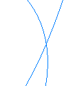
there is a pseudo-intersection between two curves if they intersect each other in the view direction
(but not really), and if the mini 3D distance between them at this cutting point is lower than
the parameter Max. Distance.
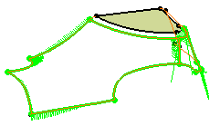
Pseudo-intersection of two curves in the view direction
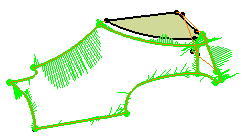
Pseudo-intersection of two curves in another view.
in the picture below, the arrows point at the minimum distance between the 2 curves.


- Deburring to remove undesirable small curve pieces, based on a Min length criterion.
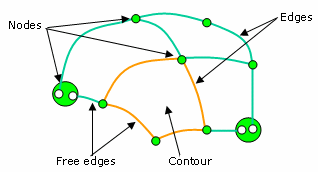
- A network is a set of closed and connected contours, named wires,
- a contour is a set of connected edges, it is necessarily closed but not limited to 3 or 4 sides,
- an edge belongs to one contour (free border edge) or 2 contours (common edge),
- if there are no free border edges, the network is closed,
- a node is the topological encounter point of two or more edges.
These edges may belong to different contours.
Once the action has detected the topology (node, contours, free border
edges),
the curves are adapted to the network internal constraints such as:
- Connection constraints on nodes
(all edges ending on a common node must be connected on this point).
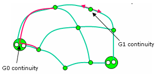
- Tangency constraints between two edges on a node.
-
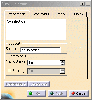
Click Curves Network
 .
The dialog box is displayed.
.
The dialog box is displayed.
-
It consists of 4 tab pages:
Stay in the Preparation tab and select the curves to clean.
They are displayed in the dialog box.
You can: - select a CleanContour, a Curves network or a Join of curves,
their curves will be added to the list. -
remove a curve from the list:
- pick the curve again in the graphic area, or
- pick the curve again in the specification tree, or
-
pick the curve you want to remove in the
list of the dialog box and
use the contextual menu Remove.
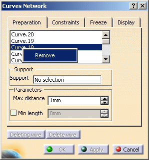
-
select additional curves, they will be added to the list.
- select a CleanContour, a Curves network or a Join of curves,
-
Select the mesh as the Support. Click Apply.
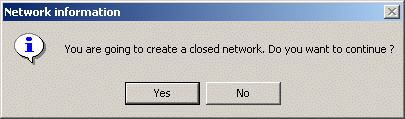
Before computing the network, the action searches overlapping curves.
If some are detected, a message is displayed: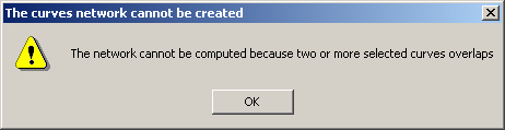
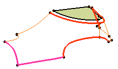
The overlapping curves are displayed in magenta 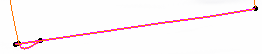
The wires are then computed and displayed. The button Deleting wire is now available. 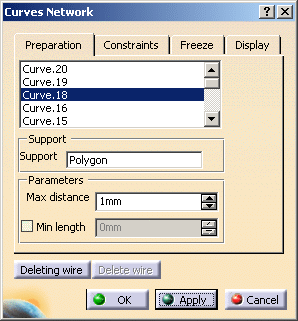
A wire is computed on each "loop" of curves, plus a large one on the "loop" formed by
the external curves because the network is considered as closed by default.
If your network does not form a closed volume, you usually do not need this large wire
(it would create an additional surface as you create surfaces from the curves network).
In the same way, you can remove wires corresponding to holes in your part.
-
Click Deleting wire to activate the wire selection. The large wire is highlighted
and a Delete wire button becomes available.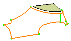
-
Click Delete wire button to remove this wire.
-
In the cases where you want to create a surface on a network of curves with a hole in it,
i.e. without filling one or several wires, use the Deleting wire button to activate the wire selection,
select the wire by picking two of its edges, and Click Delete wire. -
If you do not remove the large wire, an information message is displayed as you Click OK.
-
The parameters Max distance and Filtering are those used in the Curves Slice command.
-
Go to the Constraints tab to define constraints. The existing constraints are highlighted,
as a green dot for continuity constraints on nodes, as a blue line for tangency constraints,
as a red curve for frozen curves.
-
The constraints are applied globally on the whole network.
-
Continuity constraints on nodes are implicit and cannot be removed.
-
-
The Node tolerance defines the maximum distance between edges extremities to consider
these edges connected on a node.
You can modify this value, but it cannot be smaller than the Max distance parameter.
The Node tolerance is visualized as a green sphere whose radius is equal to the Node tolerance.
The size of this sphere is updated when you modify the Node tolerance value.
You can move the sphere using the cursor. -
Tangency constraints are activated by the Automatic tangency select box.
You can edit the value of the tangency angle. Click Apply after each modification. -
Select Projection on support to compute the network from the projections of the curves on the mesh.
The curves projected are smoothed, with the Smoothing tolerance. This parameter can be edited.
It is applied to all curves. -
You can choose between a global or a local deformation constraint
(available for all deformable edges).
This constraint is applied during the geometric adaptation step.
If the Global deformation select box is set, edges deformations are done along the entire length
of the edges.Example of global deformation: 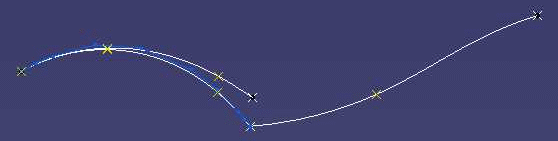
Example of local deformation: 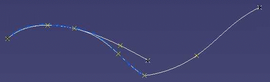
Click Default constraints to revert to the default constraints.
-
Go to the Freeze tab page to select curves that must remain frozen.
-
Pick a curve to freeze it. It is displayed in red in the graphic area and displayed in the dialog box.
Pick it again or use the contextual menu Remove to free it.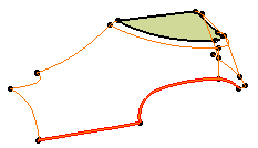
-
You can freeze only curves that have been selected in the preparation tab.
-
An edge of a face is automatically and definitely frozen.
-
Free border edges are frozen by default but you can free them.
-
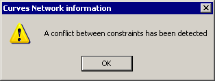
The action provides a constraint solver to search conflicts between constraints.
-
A message is displayed at the end of the search.
-
When all constraints have been selected, conflicts are highlighted in magenta.
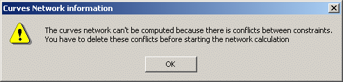
- Modify the constraints to solve the existing conflicts before creating the wires.
-
-
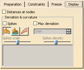
If necessary, go to the Display tab page to visualize defects or gaps on the curves.
-
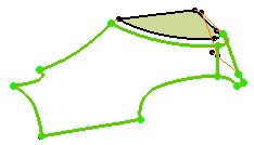
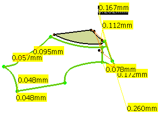
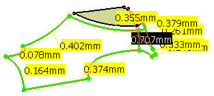
Select Distances at nodes to display the minimum 3D distance between two curves at
their pseudo-intersection.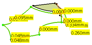
They are displayed in yellow with the exception of the greatest minimum distance found
that is displayed in black.
Click this black label to update the Max distance in the Preparation tab with a value
that will take all curves pseudo-intersection into account. -
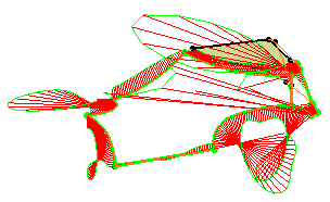
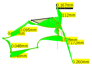
Select Spikes to display deviation or curvatures spikes:
- Click
 to display the deviation spikes between the network curves
and the input curves,
- Click
 to display the deviation spikes between the network curves
and the support mesh,
- Click
 to display the curvature spikes on the network curves.
Spikes within the tolerance are displayed in green,
spikes exceeding the tolerance are displayed in red.
- Click
-
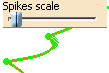
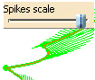
Use the Spikes scale slider to define the size of the spikes
-
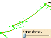
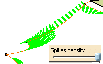
and the Spikes density slider to define their density:
-
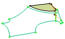
Select Max deviation and:
-
Click
to display the maximum deviation between the network curves and
the input curves,
-
Click
to display the maximum deviation spikes between the network curves
and the support mesh.
-
-
You can combine Spikes and Max deviation.
-
When Max deviation alone is selected, the greatest corresponding spike is displayed.
-
The Max deviation is not relevant for the
curvature . -
Although this is possible, we recommend that you do not combine Max deviation
with Distances at nodes as it would be difficult to read the combined information.
You should select these check boxes in turn.
-
Click OK to validate the network and exit the dialog box.
A CurvesNetwork element is created in the specification tree.
![]()