The Design of Experiments window enables you to perform virtual experiments
taking into account as many parameters as needed. It can be accessed by
clicking the Design of Experiments icon (![]() )
in the Product Engineering Optimizer workbench.
)
in the Product Engineering Optimizer workbench.
The Design of Experiments Window is made up of three different tabs:
This tab enables you to define the analysis to be performed. In this tab, you:
|
|
|
|
|
|
|
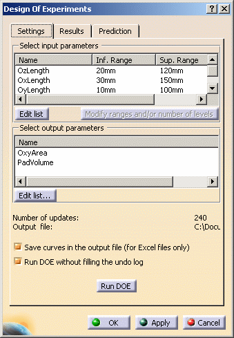 |
Select input parametersThis field enables you to select the input parameters that will be
taken into account when performing the analysis. Select an input parameter and click
Note that if you forget to check this option, and you do not want to re-run the DOE, you can generate DOE curves manually. For more information, see Useful Tips. |
This field enables you to select the output parameters (also called output factors) under consideration.
Click ![]() to access the
Select the output parameters window, select one or more parameters
by using the
to access the
Select the output parameters window, select one or more parameters
by using the ![]() button and click
OK.
button and click
OK.
To remove parameters, click Edit list... and use the arrow button to
remove them from the selected parameters and click OK.
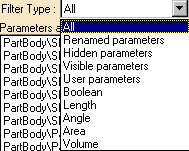 |
Note that the Filter Type scrolling list enables you to filter the type of output parameters. |
|
|
|
This tab is only available after the analysis is performed and is disabled if the information contained in the Settings tab are not up-to-date.
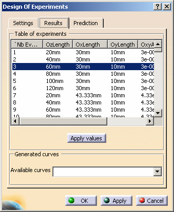 |
The matrix displayed in the Table of experiments section
is the result of computations performed for each node: the number of
evaluations presented matches the number of updates displayed in the
Settings tab.
|
The number of curves generated depends on the number of selected input and output parameters. A curve is generated:
|
|
|
Here are two curves samples (the data used to produce these curves are provided in the Using the Design of Experiments Tool topic.)
Plot of one factor effect on one output
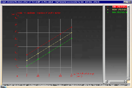 |
This graphic shows the mean effect of the 'OxLength'
parameter on the OxyPerimeter. (Click the graphic opposite to enlarge
it.)
The three curves are parallel which means that there is no interaction between the OxLength and OyLength parameters on the output parameter (OxyParameter) (i.e. the effect of OxLength on OxPerimeter does not depend on the OyLength value.) The yellow curve represents the mean. The red curve represents the mean plus 3 standard deviations. The green curve represents the mean minus 3 standard deviations. Statistically, for a given value of Ox, 99% of the values of the OXyPerimenter are located in the range between the green and the red dots. |
Plot of interaction between 2 input factors on one output
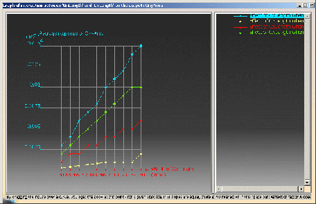 |
This graphic shows the interaction effect of the "OxLength"
and "OyLength" parameters on the OxyArea. (Click the graphic opposite to
enlarge it.)
|
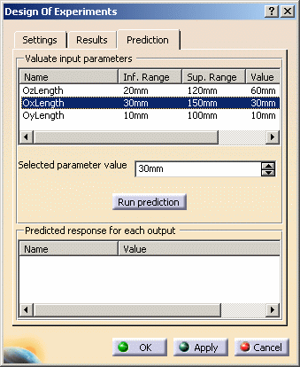 |
This tab presents a mathematical model of the system and
is used to get a theoretical value of the output parameter considering a
specific configuration of the input parameters.
|
|
|
If the result is not satisfying, refine your analysis by adding levels in the Settings tab. |
You can choose one of the 2 alternatives below to obtain predictions:
Computing the theoretical value of a node:
|
|
|
|
|
Computing the theoretical value of a node of the field of study (outside the network):
|
|
|
|
|