Useful Tips
Optimization
If you encounter a problem with many variables (more than 4) as free
parameters:
| |
- do not forget to apply ranges, and
|
| |
- begin with the gradient algorithm before trying the simulated
annealing algorithm.
|
Gradient
The gradient behaves better with squares or
quadratic functions (especially relevant for "Target Values"). Hence the
following problem:
|
Given: volume=x*y*z.
Find, x, y and z such that volume = 1000.
is better solved if the following formula is
       given to the optimizer:
objective = (volume)2
|
In most cases the properties of the functions used inside the optimization
problem are unknown. In this case, it is recommended to use the global search
algorithm (Simulated Annealing). However, as this algorithm can take a long
time to reach convergence (especially when there are many free parameters), it
could be helpful to use a local search (gradient) for a few iterations before
switching to the global search (Simulated Annealing). Eventually, when the
global search has converged and that results must be refined, reduce the ranges
around the found solution and restart a slow Local Search.
Several constraints
- Some optimization problems can contain a large number of constraints
with respect to the number of free parameters. In this case the
optimization problem can be over-constrained i.e. there is no feasible
region (set of free parameter values for which all constraints are
satisfied). The Global Search (Simulated Annealing) helps to reduce the
constraints values even in this later case. However, it does not
guarantee any access to the feasible region even if it exists.
|
- The evolution of the distances to satisfaction (that can be displayed
with the graphs) is useful to identify constraints that are difficult to
satisfy. It is sometime better to deactivate all other constraints to
identify a potential zone of satisfaction for these constraints only.
|
Recommendations
Always use well-constrained sketches when they are involved in an
optimization. Under-constrained sketches can lead to wrong solutions or
collapsed geometries (see
KwoCirclesSk.CATPart). It is also recommended to limit the ranges of the
free parameters to reasonable values.
Design of Experiments Tool
How to manually build graphics from a DoE Excel Output file?
The process described below is based on the following file:
HowToManuallyBuildGraphsFromDoEExcelOutputFile.xls
Creating the Effects Graphs:
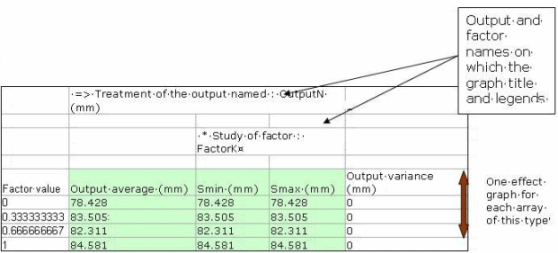
For each effect graph to build, i.e. for each array of the part
entitled ARRAYS OF FACTORS EFFECTS, for each output S and each
factor X, perform the following actions in the Excel file:
-
If not already done, open the DoE output Excel file.
-
Click the Chart Wizard command.
-
Select the Line as Chart type and click the NEXT command.
-
In the Data Range tab:
- Put the cursor in the Data Range field and select the following
highlighted range in the sheet:
|
- Check the Columns option in the Series In field.
|
-
In the Data Range tab :
- Do not modify the content of the Series frame.
|
- Put the cursor in the Category (X) axis labels field and select
the following highlighted range in the sheet :
|
|
|
-
In the Titles tab:
|
|
- Category (X) axis = VALUE of FactorK
|
- Value (Y) axis = Average of OutputN (output's
unit) responses (surrounded by min. and max. responses)
|
-
Leave the other tabs unchanged and click NEXT.
-
Choose the As Object in : Sheet1 option.
-
Click FINISH.
Creating the Interactions Graphs
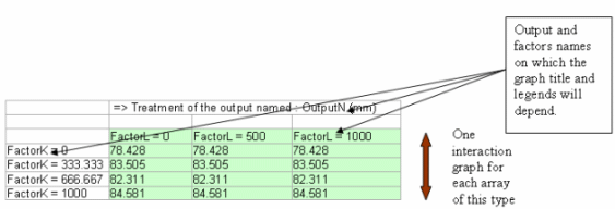
For each interaction graph to build, i.e. for each array of the
part entitled ARRAYS OF INTERACTIONS AVERAGES, perform the following
actions in the Excel file :
-
If not already done, open the DoE output Excel file.
-
Click the Chart Wizard command.
-
Select the Line as Chart type and click NEXT.
-
In the Data Range tab:
- Put the cursor in the Data Range field and select the following
highlighted range in the sheet:
|
- Check the Columns option in the Series In field
|
-
In the Series tab :
|
|
- Put the cursor in the Category (X) axis labels field and select
the following highlighted range in the sheet:
|
|
|
-
In the Titles tab :
|
|
- Category (X) axis = VALUE of FactorL
|
| (Y) axis = Average of OutputN (output's
unit) |
-
Do not modify the other tabs and click NEXT.
-
Choose the As Object in : Sheet1 option.
-
Click FINISH.
Creating the Slopes Graphs
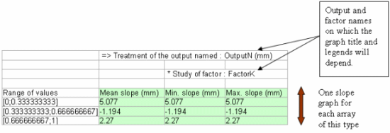
For each slope graph to build, i.e. for each array of the part
entitled ARRAYS OF EFFECTS SLOPES,perform the following actions in the Excel
file :
-
If not already done, open the DoE output Excel file.
-
Click the Chart Wizard command.
-
Select the Line as Chart type and click NEXT.
-
In the Data Range tab:
- Put the cursor in the Data Range field and select the following
highlighted range in the sheet:
|
- Check the Columns option in the Series In field.
|
-
In the Series tab :
- Do not modify the content of the Series frame
|
- Put the cursor in the Category (X) axis labels field and select
the following highlighted range in the sheet :
|
|
|
-
In the Titles tab :
- Chart Title = Mean slope of the effect curve of FactorK on
OutputN (surrounded by min. and max. slopes).
|
- Category (X) axis = Range of study = [value at level i,value at
level i+1] of factor FactorK
|
|
|
-
Do not modify the other tabs and click NEXT.
-
Choose the As Object in : Sheet1 option.
-
Click FINISH.


