You can use profiling tools to identify which portions of the program are executed most frequently or where most of the time is spent. Profilers are typically used after a basic tool, such as the vmstat or iostat commands, shows that a CPU bottleneck is causing the slow performance.
Before you begin locating hot spots in your program, you need a fully functional program and realistic data values to feed it to.
Use the timing commands discussed in Using the time Command to Measure CPU Use for testing and debugging programs whose performance you are recoding and trying to improve. The output from the time command is in minutes and seconds, as follows:
real    0m26.72s
user    0m26.53s
sys     0m0.03s
The output from the timex command is in seconds:
real 26.70
user 26.55
sys  0.02
Comparing the user+sys CPU time to the real time will give you an idea if your application is CPU-bound or I/O-bound.
Note: Be careful when you do this on an SMP system (see time and timex Cautions).
The timex command is also available through the SMIT command on the Analysis Tools menu, found under Performance and Resource Scheduling. The -p and -s options of the timex command allow data from accounting (-p) and the sar command (-s) to be accessed and reported. The -o option reports on blocks read or written.
The prof command displays a profile of CPU usage for each external symbol (routine) of a specified program. In detail, it displays the following:
The prof command interprets the profile data collected by the monitor() subroutine for the object file (a.out by default), reads the symbol table in the object file, and correlates it with the profile file (mon.out by default) generated by the monitor() subroutine. A usage report is sent to the terminal, or can be redirected to a file.
To use the prof command, use the -p option to compile a source program in C, FORTRAN, PASCAL, or COBOL. This inserts a special profiling startup function into the object file that calls the monitor() subroutine to track function calls. When the program is executed, the monitor() subroutine creates a mon.out file to track execution time. Therefore, only programs that explicitly exit or return from the main program cause the mon.out file to be produced. Also, the -p flag causes the compiler to insert a call to the mcount() subroutine into the object code generated for each recompiled function of your program. While the program runs, each time a parent calls a child function, the child calls the mcount() subroutine to increment a distinct counter for that parent-child pair. This counts the number of calls to a function.
Note: You cannot use the prof command for profiling optimized code.
By default, the displayed report is sorted by decreasing percentage of CPU time. This is the same as when specifying the -t option.
The -c option sorts by decreasing number of calls and the -n option sorts alphabetically by symbol name.
If the -s option is used, a summary file mon.sum is produced. This is useful when more than one profile file is specified with the -m option (the -m option specifies files containing monitor data).
The -z option includes all symbols, even if there are zero calls and time associated.
Other options are available and explained in the prof command in the AIX 5L Version 5.1 Commands Reference.
The following example shows the first part of the prof command output for a modified version of the Whetstone benchmark (Double Precision) program.
# cc -o cwhet -p -lm cwhet.c
# cwhet > cwhet.out
# prof
Name                 %Time     Seconds     Cumsecs  #Calls   msec/call
.main                 32.6       17.63       17.63       1  17630.
.__mcount             28.2       15.25       32.88
.mod8                 16.3        8.82       41.70 8990000      0.0010
.mod9                  9.9        5.38       47.08 6160000      0.0009
.cos                   2.9        1.57       48.65 1920000      0.0008
.exp                   2.4        1.32       49.97  930000      0.0014
.log                   2.4        1.31       51.28  930000      0.0014
.mod3                  1.9        1.01       52.29  140000      0.0072
.sin                   1.2        0.63       52.92  640000      0.0010
.sqrt                  1.1        0.59       53.51
.atan                  1.1        0.57       54.08  640000      0.0009
.pout                  0.0        0.00       54.08      10      0.0
.exit                  0.0        0.00       54.08       1      0.
.free                  0.0        0.00       54.08       2      0.
.free_y                0.0        0.00       54.08       2      0.
In this example, we see many calls to the mod8() and mod9() routines. As a starting point, examine the source code to see why they are used so much. Another starting point could be to investigate why a routine requires so much time.
Note: If the program you want to monitor uses a fork() system call, be aware that the parent and the child create the same file (mon.out). To avoid this problem, change the current directory of the child process.
The gprof command produces an execution profile of C, PASCAL, FORTRAN, or COBOL programs. The statistics of called subroutines are included in the profile of the calling program. The gprof command is useful in identifying how a program consumes CPU resources. It is roughly a superset of the prof command, giving additional information and providing more visibility to active sections of code.
The source code must be compiled with the -pg option. This action links in versions of library routines compiled for profiling and reads the symbol table in the named object file (a.out by default), correlating it with the call graph profile file (gmon.out by default). This means that the compiler inserts a call to the mcount() function into the object code generated for each recompiled function of your program. The mcount() function counts each time a parent calls a child function. Also, the monitor() function is enabled to estimate the time spent in each routine.
The gprof command generates two useful reports:
Each report section begins with an explanatory part describing the output columns. You can suppress these pages by using the -b option.
Use -s for summaries and -z to display routines with zero usage.
Where the program is executed, statistics are collected in the gmon.out file. These statistics include the following:
Later, when the gprof command is issued, it reads the a.out and gmon.out files to generate the two reports. The call-graph profile is generated first, followed by the flat profile. It is best to redirect the gprof output to a file, because browsing the flat profile first may answer most of your usage questions.
The following example shows the profiling for the cwhet benchmark program. This example is also used in The prof Command:
# cc -o cwhet -pg -lm cwhet.c
# cwhet > cwhet.out
# gprof cwhet > cwhet.gprof
The call-graph profile is the first part of the cwhet.gprof file and looks similar to the following:
granularity: each sample hit covers 4 byte(s) Time: 62.85 seconds

                                  called/total       parents
index  %time    self descendents  called+self    name           index
                                  called/total       children

               19.44       21.18       1/1           .__start [2]
[1]     64.6   19.44       21.18       1         .main [1]
                8.89        0.00 8990000/8990000     .mod8 [4]
                5.64        0.00 6160000/6160000     .mod9 [5]
                1.58        0.00  930000/930000      .exp [6]
                1.53        0.00 1920000/1920000     .cos [7]
                1.37        0.00  930000/930000      .log [8]
                1.02        0.00  140000/140000      .mod3 [10]
                0.63        0.00  640000/640000      .atan [12]
                0.52        0.00  640000/640000      .sin [14]
                0.00        0.00      10/10          .pout [27]

-----------------------------------------------
                                                     <spontaneous>
[2]     64.6    0.00       40.62                 .__start [2]
               19.44       21.18       1/1           .main [1]
                0.00        0.00       1/1           .exit [37]
-----------------------------------------------
Usually the call graph report begins with a description of each column of the report, but it has been deleted in this example. The column headings vary according to type of function (current, parent of current, or child of current function). The current function is indicated by an index in brackets at the beginning of the line. Functions are listed in decreasing order of CPU time used.
To read this report, look at the first index [1] in the left-hand column. The .main function is the current function. It was started by .__start (the parent function is on top of the current function), and it, in turn, calls .mod8 and .mod9 (the child functions are beneath the current function). All the accumulated time of .main is propagated to .__start. The self and descendents columns of the children of the current function add up to the descendents entry for the current function. The current function can have more than one parent. Execution time is allocated to the parent functions based on the number of times they are called.
The flat profile sample is the second part of the cwhet.gprof file and looks similar to the following:
granularity: each sample hit covers 4 byte(s) Total time: 62.85 seconds

  %   cumulative   self              self     total
 time   seconds  seconds     calls  ms/call  ms/call  name
 30.9      19.44    19.44        1 19440.00 40620.00  .main [1]
 30.5      38.61    19.17                             .__mcount [3]
 14.1      47.50     8.89  8990000     0.00     0.00  .mod8 [4]
  9.0      53.14     5.64  6160000     0.00     0.00  .mod9 [5]
  2.5      54.72     1.58   930000     0.00     0.00  .exp [6]
  2.4      56.25     1.53  1920000     0.00     0.00  .cos [7]
  2.2      57.62     1.37   930000     0.00     0.00  .log [8]
  2.0      58.88     1.26                             .qincrement [9]
  1.6      59.90     1.02   140000     0.01     0.01  .mod3 [10]
  1.2      60.68     0.78                             .__stack_pointer [11]
  1.0      61.31     0.63   640000     0.00     0.00  .atan [12]
  0.9      61.89     0.58                             .qincrement1 [13]
  0.8      62.41     0.52   640000     0.00     0.00  .sin [14]
  0.7      62.85     0.44                             .sqrt [15]
  0.0      62.85     0.00      180     0.00     0.00  .fwrite [16]
  0.0      62.85     0.00      180     0.00     0.00  .memchr [17]
  0.0      62.85     0.00       90     0.00     0.00  .__flsbuf [18]
  0.0      62.85     0.00       90     0.00     0.00  ._flsbuf [19]
The flat profile is much less complex than the call-graph profile and very similar to the output of the prof command. The primary columns of interest are the self seconds and the calls columns. These reflect the CPU seconds spent in each function and the number of times each function was called. The next columns to look at are self ms/call (CPU time used by the body of the function itself) and total ms/call (time in the body of the function plus any descendent functions called).
Normally, the top functions on the list are candidates for optimization, but you should also consider how many calls are made to the function. Sometimes it can be easier to make slight improvements to a frequently called function than to make extensive changes to a piece of code that is called once.
A cross reference index is the last item produced and looks similar to the following:
Index by function name

  [18] .__flsbuf            [37] .exit                 [5] .mod9
  [34] .__ioctl              [6] .exp                 [43] .moncontrol
  [20] .__mcount            [39] .expand_catname      [44] .monitor
   [3] .__mcount            [32] .free                [22] .myecvt
  [23] .__nl_langinfo_std   [33] .free_y              [28] .nl_langinfo
  [11] .__stack_pointer     [16] .fwrite              [27] .pout
  [24] ._doprnt             [40] .getenv              [29] .printf
  [35] ._findbuf            [41] .ioctl                [9] .qincrement
  [19] ._flsbuf             [42] .isatty              [13] .qincrement1
  [36] ._wrtchk              [8] .log                 [45] .saved_category_nam
  [25] ._xflsbuf             [1] .main                [46] .setlocale
  [26] ._xwrite             [17] .memchr              [14] .sin
  [12] .atan                [21] .mf2x2               [31] .splay
  [38] .catopen             [10] .mod3                [15] .sqrt
[7] .cos [4] .mod8 [30] .write
Note: If the program you want to monitor uses a fork() system call, be aware that the parent and the child create the same file (gmon.out). To avoid this problem, change the current directory of the child process.
Standard UNIX performance tools often do not capture enough information to fully describe the enhanced performance and function of the operating system. The tprof command is a versatile profiler that provides a detailed profile of CPU usage by every process ID and name. It further profiles at the application level, routine level, and even to the source statement level and provides both a global view and a detailed view. In addition, the tprof command can profile kernel extensions, stripped executable programs, and stripped libraries. It will do subroutine level profiling for most executable program on which the stripnm command will produce a symbol table.
Because activity is recorded at 100 samples per second, estimates for short-running programs might not be sufficiently accurate. Averaging multiple runs help generate a more accurate picture. The tprof command profiles only CPU activity; it does not profile other system resources, such as memory or disks.
The tprof command uses the system trace facility. Only one user at a time can execute the trace facility. Therefore, only one tprof command can be executing at one time.
Note that the tprof command cannot determine the address of a routine when interrupts are disabled. Therefore, it charges any ticks that occur while interrupts are disabled to the unlock_enable() routines.
The tprof command is described in detail in Using the tprof Program to Analyze Programs for CPU Use. The remainder of this section discusses its importance for application tuning.
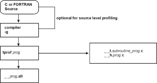
Unless profiling is desired at the source statement level, the tprof command requires no recompiling. If source level is desired, compile the C or FORTRAN source with the -g option.
The tprof command output is placed in a file called __prog.all (where prog is the name of the program profiled). If source-level profiling is indicated, additional files are created and placed in the current working directory, as follows:
The following figure illustrates source-level profiling in a flowchart:
Figure 15-1. Source Level Profiling. This illustration is a flowchart beginning with a box labeled C or FORTRAN Source. The data path goes down to a second box labeled compiler --g. The path continues down to the next box labeled tprof prog. From here the path can go 2 directions. It can go to the last box labeled __prog.all, or a side box labeled __t.subroutine_prog.c and __h.prog.c. The first 2 boxes are optional for source level profiling.
|
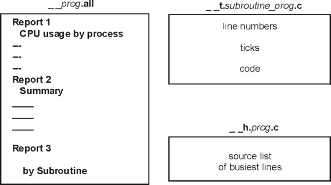
When the tprof command is used, one report is always produced: a summary report with the .all suffix. This first section contains an estimate of CPU time spent in each process while the program or command was executing. The report shows CPU time, as well as the amount of idle and kernel time.
The second section in the .all file summarizes the first section by process. The third section in the .all file shows the detail at the subprogram level.
The following figure illustrates the most important files generated and their contents:
Figure 15-2. tprof Reports. This illustration depitcs files generated by the tprof command. The first file is __prog.all and it contains 3 reports. Report 1 lists CPU usage by process. Report 2 is a summary. Report 3 reports use by subroutine. The next file is the __t.subroutine_prog.c file. This file contains line numbers, ticks, and code. The last file is the __h.prog.c file. This file contains a source list of the busiest lines.
 |
For an example of the tprof command output, see A tprof Example.