Specifying the Algorithm to Be Run

Types of Algorithms

To perform an optimization, you can use one of the following algorithms:

User Algorithm defined in CAAOptimizationInterfaces.edu

Local Algorithm for Constraints and Priorities:
A Gradient based search using a modified feasible direction.

Simulated Annealing Algorithm

Algorithm for Constraints & Derivatives Providers:
A gradient based search for features that provide their own derivatives such as some analysis sensors.

Gradient Algorithm without Constraints:
3 different types of gradient algorithms:

Fast: A successive quadratic interpolation that allows fast but less accurate optimization.
Medium: A randomly restarted conjugate gradient.
Slow: A steepest descent algorithm (slow but more accurate than the Fast category).

Gradient Algorithm with Constraints:
A gradient based feasible direction algorithm.

User algorithm defined in CAAOptimizationInterfaces.edu

You can define your own algorithms. To get an example, See the CAAOptimization interfaces.

Local Algorithm for Constraints & Priorities

This algorithm takes constraints priorities into account.

Simulated Annealing Algorithm

This algorithm is a global stochastic search algorithm hence two successive runs of this method might not lead to the same result. It performs a global search that evolves towards local searches as the time goes on.
It is usually used to explore non-linear, multimodal functions. These functions can also be discontinuous.
If the shape of the objective function is unknown, it is recommended to start with a Simulated Annealing then refine the results with a gradient descent. This approach is slow but works for a larger amount of functions.

A good way to quickly reach a solution when using the Simulated Annealing consists in specifying a low number of consecutive updates without improvements (15 or 20).
On the contrary, to foster search, the number of consecutive updates without improvements can be increased as well as the time and the number of total updates.

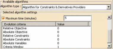
Algorithm for Constraints & Derivatives Providers

This algorithm can handle objectives providing derivatives (like analysis global sensors) in conjunction with constraints providing multiple values and derivatives (like analysis local sensors). With this algorithm additional termination criteria can be specified:

Criteria Window: Number of updates (Nstop) with respect to which the termination criteria will be evaluated.
Relative Constraints: Relative constraints variation under which the algorithm must stop. All constraints must fulfill this criteria for the stop to occur.
Absolute Constraints: Absolute constraints variation under which the algorithm must stop. All constraints must fulfill this criteria for the stop to occur.
Absolute Variables: Absolute variables variation under which the algorithm must stop. All variables must fulfill this criteria for the stop to occur.

`Absolute Objective`: Absolute objective variation under which the algorithm must stop. (See formula opposite)	`Obj._Max.-Obj._Min < User Termination Criteria`
`Relative Objective`: Relative objective variation under which the algorithm must stop (See formula opposite)	`Obj._Max-Obj._Min _______________ Obj._max+Obj._min ________ 2`	Where: Obj. Max is the maximum objective value obtained during the "criteria window". Obj. Min is the minimum objective value obtained during the "criteria window".

Gradient algorithm

This algorithm must be used first to perform a local search. Based on the calculation of a local slope of the objective function, this algorithm will use a parabolic approximation and jump to its minimum, or use an iterated exponential step descent in the direction of the minimum.
If the properties of the objective function are known (continuous, differentiable at all point), the gradient can be used straight on. It is usually faster than the Simulated Annealing algorithm.

You can choose to run the Gradient algorithm with constraints or without constraints.

Global Search vs. Local Search

Simulated Annealing (Global Algorithm)	Gradient (Local Algorithm) Local Algorithm For Constraints & Priorities, Algorithm for Constraints and Derivatives Providers, Gradient Algorithm Without Constraint, Gradient Algorithm With Constraint(s)
Equality constraints allowed Precision is managed as a termination criteria. x == A is fulfilled when abs(x - A) < precision	Equality constraints not allowed except for the Algorithm for Constraints and Derivatives Providers.
Can be run with constraints and no objective function	Must be run with an objective function.

Algorithms Configurations

The Gradient algorithms, the Simulated Annealing algorithm, and the Algorithm for Constraints & Derivatives Providers can be run in 3/4 different configurations.

`Options`	`Gradient Algorithm`	`Simulated Annealing Algorithm`	`Algorithm for Constraints & Derivatives Providers`
Slow	Slow evolution based on the steepest descent algorithm and on steps. Good precision (to be used to find convergence.)	These 4 configurations define the level of acceptance of bad solutions. If the problem has many local optima, use Slow. If the problem has no local optima, use Infinite (Hill climbing).
Medium	A randomly restarted conjugate gradient.
Fast	Search jumps from Minimum to Minimum using quadratic interpolation. Fast evolution, less precision.
Infinite (Hill climbing)	-

Termination Criteria

Termination criteria are used to stop the optimizer. When an optimization is running, a message box displays the data of each update. You can stop the computation by clicking Stop. If you don't intervene in the computation process, the computation will stop:

	When a value (minimum, maximum or target value) has been found and the algorithm is unable to progress anymore (Gradient.) or
	When one of the specified termination criteria has been met.

Here are the termination criteria to be specified:

	Maximum number of updates i.e. the number of times the objective function will be calculated at most (number of updates.)
	Number of updates without improvement i.e. the number of updates allowed without achieving a better result.
	Maximum duration of computation

Simulated Annealing always runs until one of the termination criteria is reached. The Gradient can stop before if a local optimum is reached.

Algorithms Summary

Please find below a table listing the available algorithms along with the functions they support.

	`Local Algorithm for constraints and priorities`	`Simulated Annealing Algorithm`	`Algorithm for Constraints and derivatives providers`	`Gradient without constraints`	`Gradient with constraints`
Inequality Constraints	Yes	Yes	Yes	No	Yes
Equality Constraints	No	Yes	Yes	No	No
Priorities on constraints	Yes	No	No	No	No
Derivatives providers	No	No	Yes	No	No
Non Differentiable objectives or Constraints	No	Yes	No	No	No

Algorithms Versions

From time to time, the PEO algorithms are updated to enhance their performance. The side effect of these modifications is a change of behavior of the optimization process. It is however possible to come back to the previous versions of the algorithms by using environment variables (see table below.)

`Var Name`	`Var Value`
GradientVersion	r8Sp3, r9sp4, r10sp1, r11ga
SAVersion	r8sp3, r13ga, r14ga, r14sp1
GradientWithCstVersion	r8sp4, r11ga, r13ga, r14ga, r14sp1, r14sp2, r15ga, r16ga*
^*A pop-up is displayed at the end of the optimization run when the bound of at least one free parameter is reached.