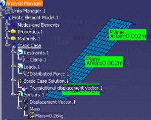
- In the scenario described below, you want to find out the total plate thicknesses that will enable you to minimize the plate mass and that satisfies a displacement constraint. Note that the plate is made up of 3 different plates (thickness=2mm). The plate is screwed to a wall and a distributed force is exerted at the opposite extremity.
- You want to minimize the plate mass by modifying each plate thickness.
- The displacement vector of each meshing node must be inferior to 0.2mm.
- To use the Algorithm for Constraints & Derivatives Providers, you must be familiar with objects and constraints providing their own derivatives.
- To perform this scenario, you will use the Algorithm for Constraints & Derivatives Providers. For more information about it, see Specifying the Algorithm to be Run.
- To perform this scenario, you must be familiar with local and global sensors. For more information about those sensors, see Generative Structural Analysis User's Guide: User Tasks: Creating Local Sensors.
|
|
|
|
![]()
-
Open the KwoDedicatedAlgoforDerivativesProviders.CATAnalysis file.
-
Make sure the sensors are updated.
- From the Start>Analysis&Simulation menu, access the Generative Structural Analysis workbench.
- Click the Compute icon (
 ).
The Compute dialog box is displayed. Click OK.
).
The Compute dialog box is displayed. Click OK.
- Click Yes in the Computation Resources Estimation: The sensors are updated.
-
From the Start>Knowledgeware menu, access the Product Engineering Optimizer workbench.
-
Click the Optimization icon (
 ).
The Optimize dialog box is displayed.
).
The Optimize dialog box is displayed. -
In the Optimization type list, select Minimization.
-
In the Optimized parameter field, click Select.... and select the Mass parameter. Click OK.
-
In the Free parameters field, click Edit list and select the following parameters:
- Finite Element Model.1\2D Property.3\SAMThickness
- Finite Element Model.1\2D Property.2\SAMThickness
- Finite Element Model.1\2D Property.1\SAMThickness
-
Select the Finite Element Model.1\2D Property.3\SAMThickness free parameter and click Edit ranges and step. In the dialog box, enter the inferior range: 0.1 and the superior range: 30mm. Click OK when done.
-
Repeat this step for Finite Element Model.1\2D Property.2\SAMThickness and Finite Element Model.1\2D Property.1\SAMThickness.
-
In the Algorithm type, select the Algorithm for Constraints & Derivatives Providers.
-
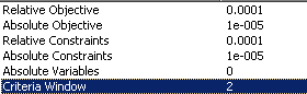
In the Termination Criteria field, set the settings as follows:
- Maximum number of updates: 10
- Consecutive updates without improvements: 7
- Maximum time: 5
-
Set the evolution criteria as follows:
-
Check the Save optimization data option.
-
In the Constraints tab, click New (derivatives provider). In the Optimization constraints editor, enter the following constraint body and click OK when done:

-
Click Run optimization. Enter the name of the .xls output file and click Save.
-
Click the Computation Results tab. The sorted results are displayed. The best result mass is 0.265675157 (Constraint: -3.27e-008).
-
Select the appropriate line and click Show Curves... The curves are displayed. The yellow line shows the mass curve and the red one shows the constraint.
![]()