About sensors:
This functionality enables to visualize all joint values (with commands
or not), measures and joint limits if defined throughout the simulation
process.
These different values used as sensors provide useful information to check
your mechanism design through both kinematics simulation operations (i.e.
simulation with laws and simulation with commands)
Within a simulation with laws, you can not only plot sensors with respect a time parameter, but you can also plot a sensor with respect to another sensor.
-
Click the Simulation with Laws icon
 in the DMU Kinematics toolbar.
The Kinematics Simulation -Mechanism.1 dialog box is displayed. -
Change the simulation duration, click the Edit Time range button
 . The Simulation
duration is automatically displayed. The default duration is 10 s
 -
Enter 20 s in the maximum time bound field:

-
Change the step number to 200.
-
Select the Activate Sensors check box.
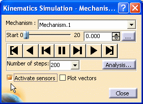
This scenario aims at checking the motion of the valve with respect to the crankshaft You are going to check if your Kinematics mechanism is correctly designed using the corresponding sensors during simulation
-
Select the sensors to be observed in the Sensors dialog box.
-
Prismatic.25
-
Revolute.18
-
Revolute.5
Launch the Simulation With laws -
-
Click the History tab to visualize the sensors behavior while running your simulation:
Use the Play Forward button
-
Click the Options button
 .
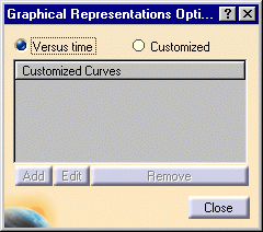
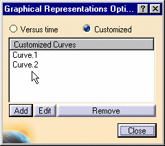
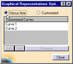
.The Graphical Representation Options dialog box is displayed:
-
Select the Customized option button: the Add, Edit and Remove buttons become accessible.

-
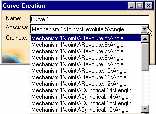
Click Add, the Curve Creation dialog box is displayed

-
In the Abscissa and Ordinate lists, select the required sensors:
-
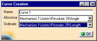
Create two customized curves:
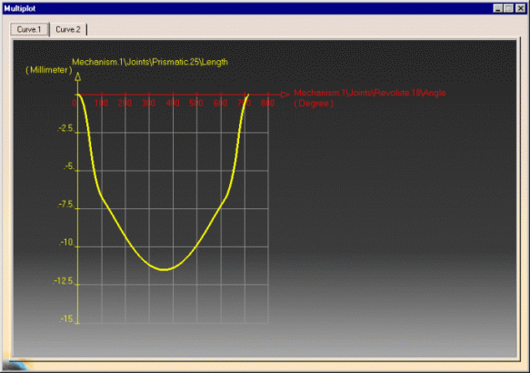
- curve1: prismatic 25 with respect to Revolute18
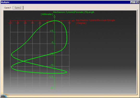
- curve2: prismatic 25 with respect to Revolute 5
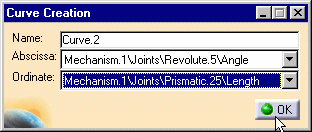
(Optional)
Give a meaningful name to your new customized curve. -
Click Ok when done.The two curves are created:
-
Click Close.
-
Click the Graphics button from the outputs to obtain a graphical representation. The curve 1 is displayed
-
Click Curve.2 tab:
-
Click File to save as a .xls or .txt file.
Give a name and a path.
Note: you can swap to the default mode (curves plotted with respect to time) at any time -
Click the Options button and select the versus time option button
-
Click Close
-
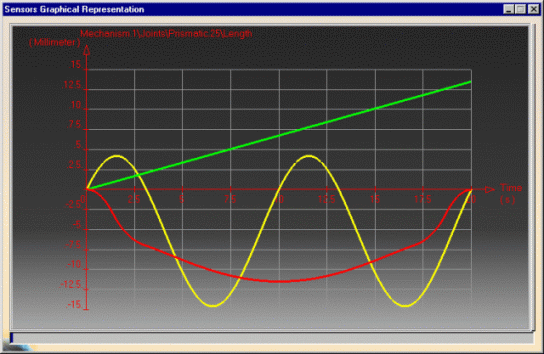
Click again the Graphics button from the outputs to obtain a graphical representation
![]()